Neurons for Dummies - 1

If you have ever heard about neural networks and thought: "how the heck do they learn?" you have landed in the right place.
Let's start immediately with a fresh spoiler of the day: there is no magic, just tons of multiplications, sums, and derivatives.
In this article, I want to tell you with calm and without panic, what happens inside an artificial neuron and how it learns from its mistakes, and we will do it step by step, with a practical example.

Anatomy of a Neural Network

Before understanding how a neural network works, we first need to clarify what a neural network actually is. Let's start by saying that there are different types of neural networks: convolutional, recurrent, and many others. One or the other is chosen depending on the problem to be solved. In this article, we will focus on Multi Layer Perceptron networks (or MLP), which are usually represented like this:

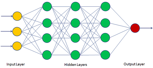Figure 1. Multi Layer Perceptron

The image may look simple, but behind that simplicity hides a number of concepts enough to make you want to commit harakiri.
And from this plethora of concepts... we will only scratch the surface. Let's start by talking about what we have in front of our eyes:

• Writings
• Arrows
• Dots

Each little ball is called a neuron (or perceptron), and as you can see, they are arranged into layers (or, if you prefer, strata). Each layer is fully connected to the next — meaning: all the neurons in one layer are linked to all the neurons in the next layer. This already explains why these architectures are called MLP, or Multi Layer Perceptron. There are three types of layers:

• Input Layer: Takes the data we provide as input. In the image, it is the yellow layer.
• Hidden Layer(s): They are called this because we don't interact with them directly. Their job is to forward propagate the processed data. In the image, they are the green ones.
• Output Layer: Contains the result. In the image, it is the red layer.

To give a practical example, let's suppose we can't recognize whether a picture shows a dog or a cat (and I sincerely hope this is just a supposition), we feed our picture into the input layer, which receives the data. This data is then processed by the hidden layers, and finally we get the result — dog or cat — in the output layer.
But before the network can say "dog" or "cat," it needs to be trained. Training a neural network simply means giving it lots of pictures of dogs and cats, and correcting it every time it makes a mistake, in order to adjust the aim for future predictions. If you’ve made it this far, you might be wondering: "Ok, but how...?" Hold your horses, cowboy — we’ll get there.

From the Network to the Neuron

We have talked about networks, layers, arrows, and dots.
But to truly understand how a neural network makes decisions (and how it learns from its mistakes), we need to go down a level. Down to the level of the dot.
Let's start by looking at the stylization of a biological neuron.

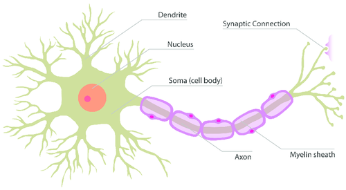Figura 2. Biological Neuron

In life, I have few certainties, but one of them is that I am not a neurologist, so I hope the experts will forgive the simplification that follows. The dendrites are stimulated by incoming electrical signals. The nucleus, together with the soma, processes the information, and the axon propagates it toward the synaptic connections, linking to the next neurons.

Does it ring a bell?

Now that we know how a biological neuron "works" (yes, the quotation marks are intentional), let's take a big leap of imagination and see how an artificial neuron is represented, the now famous little dot:

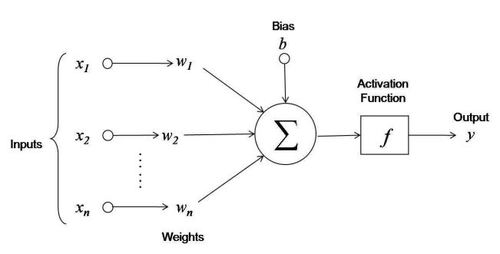Figura 3. Artificial Neuron

From this image, we can introduce many of the concepts necessary for our purpose:

• Input: these are the neuron's inputs, meaning what stimulates the dendrites.
• Weights: they are numerical values that indicate how important a particular input is. The higher the weight, the greater the influence of the input. Spoiler: the weights are the heart of everything, as we will soon see.
• Transfer Function: it serves to combine all the separate inputs into a single value. It is the equivalent of what the nucleus and soma do.
• Activation Function: it transforms the result of the transfer function. The output is connected to the neurons of the next layer, somewhat like the axon in biological neurons.
• Bias: it is a pure number whose role we will soon explain.

Putting all the individual pieces together, we have that: the inputs \(x_i\) and the weights \(w_i\) pass through the transfer function \(H\), defined as:

performing what is called a weighted sum: each input is multiplied by its weight, everything is summed up, and the bias is added.
The result of the weighted sum is then passed through the activation function \(\sigma(H)\).
The output of the single neuron is therefore:

There are many activation functions, and their selection depends on various technical factors.
While it would be worth dedicating a full article to them, for now it’s enough to know that they are fundamental for introducing non-linearity.
Which, for friends, simply means: without them, the network wouldn't even be able to correctly predict a dog from a cat.

Confused?

I would be surprised if you weren't. But don't worry, because now we have all the ingredients to see how a neuron works mathematically, and everything will become much clearer with a numerical example.

A Numerical Example. The AND Problem.

Let's start this new paragraph by introducing the problem to solve, the AND problem. The AND between two binary variables is a simple logical operation: the result is \(1\) only if both variables are \(1\) in all other cases, it is \(0\). To be more formal, let's consider two variables \(A \in \{0, 1\}\) and \(B \in \{0, 1\}\) the result of \(AND(x_1, x_2)\) is summarized in the following table, called the truth table:

Here we presented the simplest case of the AND problem, but there’s no restriction on the number of variables.
For example, with three variables, we would get the following truth table:

Let's now consider a neural network, the simplest possible: composed of a single perceptron. The goal is to solve the two-variable AND problem, that is: given the inputs \(x_1\) and \(x_2\), predict what the output of \(AND(x_1, x_2)\) which can be \(0\) or \(1\). Since the output can take only two distinct values, either salt or pepper, the problem we are dealing with is a typical classification problem.

Good: we have defined the problem and the architecture of the neural network.
Now, three things remain to be established:

1. How many inputs do we have?
2. What are the values of the weights and the bias?
3. What is the activation function?

Let's answer right away:

1. The number of inputs depends on the variables of the problem. Since the AND problem is two-variable, also called features in the context of Machine Learning, the neuron will have two inputs \(x_1\) e \(x_2\), whose values can be \(0\) o \(1\).
2. At this stage, we will assign the weights and bias ourselves. Let's suppose that:
   • the weight related to the input \(x_1\) is \(w_1 = 0.5\),
   • the weight related to the input \(x_2\) is \(w_2 = 0.5\),
   • the bias is \(b=1\).
3. We choose the Heaviside step function as the activation function

The Heaviside step is a simple function whose graph is as follows:

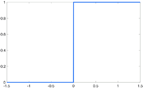Figura 4. Heaviside Step

In short, given any value \(x\) as input, the Heaviside step function returns:

• \(0\) if \(x < 0\),
• \(1\) otherwise.

Mathematically:

Why the Heaviside step function, you might be wondering?
Well, as mentioned earlier, there are many technical factors to consider, but suffice it to say that it’s the one that best fits our purpose:
the problem requires a solution that is either \(0\) o \(1\), and the Heaviside step function returns exactly an output of \(0\) o \(1\). I'd say it's a perfect match, wouldn't you agree!? But nope. For now for the sake of simplicity, we’ll settle for this, and the reason why... we’ll discover it later.

At this point, all that's left is to see how a neural network makes its predictions. And how do we see it? With a simple substitution of variables.
There are four possible cases. Remember that

that \(w_1 = 0.5, w_2 = 0.5, b = 1\) and \(\sigma(H) = 1\) only if \(H \geq 0\)

We have:

• Case 1: \(x_1 = 0, x_2 = 0\) \(H= 0 \cdot 0.5 + 0 \cdot 0.5 + 1 = 1 \Rightarrow p = \sigma(H) = \sigma(1) = 1\)
• Case 2: \(x_1 = 1, x_2 = 0\) \(H= 1 \cdot 0.5 + 0 \cdot 0.5 + 1 = 1.5 \Rightarrow p = \sigma(H) = \sigma(1.5) = 1\)
• Case 3: \(x_1 = 0, x_2 = 1\) \(H= 0 \cdot 0.5 + 1 \cdot 0.5 + 1 = 1.5 \Rightarrow p = \sigma(H) = \sigma(1.5) = 1\)
• Case 4: \(x_1 = 1, x_2 = 1\) \(H= 1 \cdot 0.5 + 1 \cdot 0.5 + 1 = 2 \Rightarrow p = \sigma(H) = \sigma(2) = 1\)

Let's now repeat the truth table, also showing the predictions made by the created perceptron, with incorrect ones highlighted in red and correct ones in green:

As we can see, our perceptron made only one correct prediction out of four. We can say it without mincing words: it sucks quite a bit, right?! So why all this fuss to reach such a poor result? Simple: because this is just the foundation.
Now, we still need to understand how to improve the results — that is, how to train the neural network so that it stops sucking and starts making sensible predictions...
But in the meantime, you've already achieved an important milestone:
Now you know that the "magic" behind predictions, or at least a good chunk of it, isn't that magical after all.

To Wrap Up

Let me say goodbye with this short code snippet, which simply replicates exactly what we have seen together.

# Definition of the Heaviside step function
class Heaviside(Activation):

    def __call__(self, x) -> int:
        result = 1
        if x < 0:
            result = 0
        return result

# Definition of the perceptron
class Perceptron:

    def __init__(self, dimension: int, activation: Activation = None):
        self._weights = np.zeros(dimension)
        self._bias = 0.
        self._activation = activation

    def __call__(self, inputs: np.ndarray) -> float:
        weighted_sum = np.dot(inputs, self._weights) + self._bias
        result = weighted_sum
        if self._activation is not None:
            result = self._activation(weighted_sum)
        return result

# Code execution
perceptron = Perceptron(dimension=2, activation=Heaviside())
perceptron.weights = np.array([0.5, 0.5])
perceptron.bias = 1.

cases = [[0, 0], [0, 1], [1, 0], [1, 1]]
true = [0, 0, 0, 1]
for i, (case, y) in enumerate(zip(cases, true)):
    prediction = perceptron(inputs=np.array(case))
    print(f"Case {i + 1}. Input = {case}, True Result = {y}, Predicted Result = {prediction}")

The output should be as follows:

Case 1. Input = [0, 0], True Result = 0, Predicted Result = 1
Case 2. Input = [0, 1], True Result = 0, Predicted Result = 1
Case 3. Input = [1, 0], True Result = 0, Predicted Result = 1
Case 4. Input = [1, 1], True Result = 1, Predicted Result = 1

If you're curious, I invite you to check out the full code here.

And to wrap it up... you thought I had forgotten, didn't you?! That I had sold you some nonsense. But no, my friends, I invite you to read the second part. Surely you don't want to stop at just how the network predicts, right?! You can't live without knowing how it learns. Yes, I know, I'm worse than the De Agostini magazine series... but that's how it is. While waiting for the second part, I bid you farewell.

Until next time.