

Here we are again for the second part of the article devoted to the neuron.
If you landed here by mistake... RUN AWAY!
Just kidding, of course you’re invited to read the first part here.
That said, in the first part I left you with more questions than answers. Today we’ll finally try to clear things up a bit.
Understanding Where Things Go Wrong
Let's begin this section by recalling one fundamental point: the weights are at the center of everything. Why!?
Because they’re the only thing we can modify. We certainly can’t change the input, that comes from the problem itself and
we have to take it as is. So, if we want to change the value of the transfer function, and therefore the output, we must act on them.
Keeping this premise in mind and bearing in mind the predictions we made in part one, our goal is to move from these results:
to these:
In other words, we want every prediction to be correct or, to put it more technically, we want the prediction error to be as small
as possible. So the first thing to do is obvious: measure the error.
To do that we need to define a Loss Function (also called an Error Function), that is something that tells us how far we are from the
ideal situation, which, for simplicity, we’ll consider to be the one where the error equals zero.
There are plenty of loss functions, each designed for a specific type of problem. In our case—remember, we’re dealing with the AND problem, we’re facing a binary classification task, so the most suitable choice is the Binary Cross Entropy - BCE.
Let’s write down the formula:
where:
- \(\ln(\cdot)\) natural logarithm
- \(y_i\) the ground‑truth label for the i‑th input
- \(p_i\) the probability predicted by the perceptron for that same input
Applying this formula to the following truth table:
For the first row we have:
\(y_0 = 0, p_0 = 1 \ \Rightarrow\ BCE_0 = -[0 \cdot \ln(1) + (1 - 0) \cdot \ln(1 - 1)] = -\infty\)
As you can see, the error is maximal and indeed, the prediction is the exact opposite of the real result.
Applying it to the last row instead:
\(y_3 = 1,; p_3 = 1 \ \Rightarrow\ BCE_3 = -[1 \cdot \ln(1) + (1 - 1) \cdot \ln(1 - 1)] = 0\)
Here the error is zero because the prediction is exactly as expected.
Adding up all the error components we obtain the total error:
\(BCE = \sum_{i}{BCE_i}\)
But watch out: in this case the error turns out to be infinite, which may make sense... or not. Don’t worry, we’ll fix that detail soon. For now, let’s keep going.
Now that we’ve introduced the concept of error, it should be clearer why the weights are truly at the heart of everything.
Remember when I told you they’re the only point we can intervene on? Good...
Now the real question is: how do we change the weights so that the error is as small as possible?
Learning, in the context of neural networks, means answering exactly that question. And we want the weights to be updated automatically,
otherwise what kind of artificial intelligence would it be!?
So, mathematically speaking, what tool lets us minimise (or maximise) a multivariable function?
Okay, I admit it’s a tough question if you’re not familiar with mathematical analysis. So I’ll spare you and give you the answer straight
away without too much sweat. We’re talking about the Gradient, or, for the more riotous among you, the vector of Partial Derivatives.
Denoting the loss function by \(L\) and a generic weight by \(w_i\), we can write:
Yes, I know, it looks like gibberish. And maybe right now you want to hit me. But in reality what each component is saying,
in plain terms, is very simple:
How much does a generic \(w_i\) affect the error value if I tweak it?
And looking at the entire gradient, the question becomes:
What should the individual \(w_i\) values be in order to reach the minimum (or maximum) of the error?
If you think the complexity ends here... sorry to disappoint you, there are still a couple of steps to tackle.
Err, Err, Err… I Prefer to Repair
Just because we like to complicate our lives, let’s recap the entire chain of calculations a perceptron performs, from input all the way to the error measurement:
- We compute the weighted sum of the inputs via the transfer function: \(net = H(x_i, w_i)\)
- We compute the prediction by applying an activation function \(\sigma\) to the output of the transfer function: \(p = \sigma(net) = \sigma(H(x_i, w_i))\)
- We compute the error by feeding the activation output into a loss function \(L\): \(loss =L(p) = L(\sigma(net))=L(\sigma(H(x_i, w_i)))\)
Hence, the entire chain is represented by the formula: \(L(\sigma(H(x_i, w_i)))\) From the previous paragraph you also know that:
- We want to minimise \(L\).
- We do so by differentiating with respect to the weights.
Mathematically, that means writing:
To differentiate this monster we need the chain rule. Far be it from me to write a treatise on analysis, if you want a quick explanation you can find one here. Applying the rule to our composite loss function we get:
where:
- \(\frac{\partial L }{\partial p}\): is the derivative of the loss with respect to the prediction.
- \(\frac{\partial p }{\partial net}\): is the derivative of the activation function with respect to the transfer function output.
- \(\frac{\partial net }{\partial w_i}\): is the derivative of the transfer function with respect to a given weight \(w_i\).
Folks, we’re almost there, the finish line is in sight. One last conceptual push...
We know how to compute the error.
We know how to express it as a function of the weights.
Now all that’s left is to minimise it.
At school, in high school, at university, they teach you that to find a minimum (or a maximum) you use the first derivative,
and that’s obviously true analytically speaking. I’m not going to rewrite the rules of mathematics. But let me ask you a question...
How could we minimise, analytically, a function with millions of parameters? Because yes, that’s exactly what happens:
we want to minimise the error, but that error is a function that depends on millions of weights. I’m being nice and showing you the
example with just one perceptron... but in reality there are hundreds and hundreds of perceptrons arranged over multiple layers, each with many inputs.
Not only would we have no idea how to calculate it, we’d take forever, and there’s no guarantee a global minimum even exists.
So I ask you: is it worth it?
And this is where numerical methods come into play.
They may not be as elegant as analytical methods but, darn it, they work.
We thus arrive at the final ingredient of this lavish dish: Gradient Descent. Within machine learning it's one of many Optimizers.
The underlying idea is simple, and let me explain it with the most overused metaphor: the blindfolded climber.
Imagine you’re on a mountain, blindfolded, and your goal is to descend to the valley.
How do you proceed?
If you feel the ground rising in one direction, you head in the opposite direction, and you do so in very small steps,
because you’re blindfolded and don’t know the terrain (and hopefully you’re not planning to sprint downhill blindly... right?).
What you’re doing is essentially a series of local checks, step by small step, not a global one, because a global approach would require perfect knowledge of the mountain, and you’re blindfolded.
That’s exactly what gradient descent does: it proceeds in tiny steps because we lack global knowledge of the loss function but we know locally, with the current weights, how we’re doing.
In formula form it’s written:
where:
- \(w_i^{new}\): the new weight after making a small adjustment. The current one the climber’s new position.
- \(w_i\): the current weight. The climber's current position.
- \(\eta\): the learning rate, indicating by how much to change the weight. It's the size of the climber’s step. If \(\eta = 0\) the climber stands still and the new weight equals the old one. If \(\eta\) is too large it's dangerous because you don’t know where you’re stepping, mathematically it means overshooting the region where the error was low.
- \(-\frac{\partial L }{\partial w_i}\): the derivative of the loss with respect to the weight that is, the direction in which the error increases or decreases.
The minus sign means we want to move in the direction that reduces the error. It represents the climber’s ability to guess where the slope goes down
and where it goes up. Indeed:
- If \(\frac{\partial L }{\partial w_i} > 0\): as \(w_i\) increases, the error increases, so we want \(w_i^{new}\) to decrease.
- If \(\frac{\partial L }{\partial w_i} < 0\): as \(w_i\) increases, the error decreases, so we want \(w_i^{new}\) to increase.
Graphically we can picture it as an entity that always aims for the lowest areas of the plot.
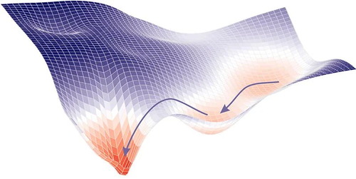 Figure 1. Gradient Descent
If you want a very broad overview of how we arrive at the gradient‑descent formula, check out this section, otherwise skip ahead and we'll (finally!) look at a numerical example.
Back to the Fut...Uhm to the AND Problem
And here we are, folks, finally ready to see how a neural network learns. Remember the AND problem? If so go right ahead, if not, refresh your memory here. Didn’t I warn you not to get attached to the Heaviside step? It’s time to ditch it. You know what they say: an activation dies, another one rises, and we’re taking the Sigmoid function. Curious why Heaviside isn’t suitable? Take a look here.
The sigmoid is defined as:
and it looks like this:
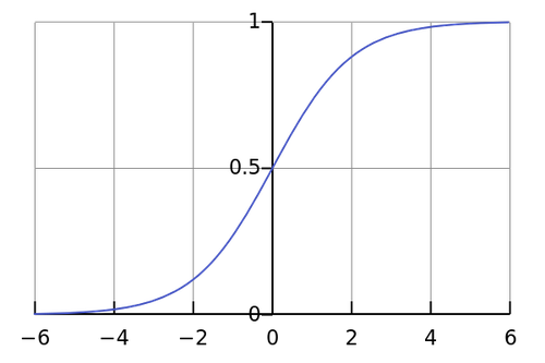 Figure 2. Sigmoid Function
As you can see, its output is always in the range \((0, 1)\).
Feed it \(x = \infty\)? The sigmoid doesn’t care, it gives you \(1\).
Feed it \(x = -\infty\)? The sigmoid doesn’t care, it gives you \(0\).
The sigmoid is too strong. Don’t challenge the sigmoid because you’ll lose anyway.
Arm‑wrestling aside, you’ll agree the sigmoid is the ideal function to represent a probability. After all, a probability is nothing more than a decimal number between \([0, 1]\) where:
- \(1\) means definitely yes
- \(0\) means definitely no
- \(0.5\) means meh
Now that we’re experts on sigmoids, let’s pick up our trusty perceptron:
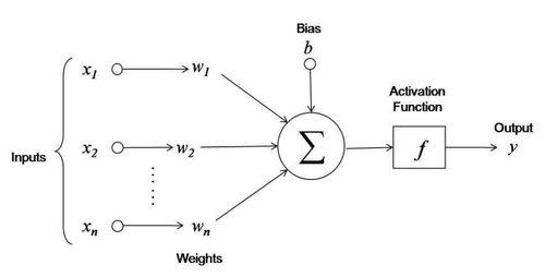 Figure 3. Artificial Neuron
and recall our weights and bias:
- \(w_1 = 0.5\)
- \(w_2 = 0.5\)
- \(b=1\)
Consider the case \(x_1 = 0, x_2 = 1 \Rightarrow y=0\) The activation output is: \(net = 0 \cdot 0.5 + 1 \cdot 0.5 + 1 = 1.5\) therefore: \( p = \sigma(1.5) \approx 0.817\) We want the derivative of the loss with respect to the weights (and the bias), namely:
We already know how to compute the loss, right? We introduced Binary Cross‑Entropy (BCE) precisely for that. So let’s see step by step what really happens.
- \(\frac{\partial L }{\partial p}\): is the derivative of the loss with respect to the prediction. From calculus, for BCE it is:
$$\left( \frac{y}{p} + \frac{ 1 - y}{ 1 - p} \right)$$Plugging in \(p = 0.817\) and \(y = 0\), we get:$$\left( \frac{0}{0.817} + \frac{ 1 - 0}{ 1 - 0.817} \right) \approx 5.481$$
- \(\frac{\partial p }{\partial net}\): is the derivative of the activation with respect to the transfer output. For the sigmoid:
$$\frac{\partial p }{\partial net} = \sigma(net) \cdot (1 - \sigma(net)) = p \cdot (1 - p)$$Plugging in \(p=0.817\), we get:$$\frac{\partial p }{\partial net} = p \cdot (1 - p) = 0.817 \cdot (1-0.817) \approx 0.149$$
- \(\frac{\partial net }{\partial w_i}\): is the derivative of the transfer function with respect to a weight, and calculus tells us:
$$ \frac{\partial net }{\partial w_i} = \frac{\partial (x_1 \cdot w_1 + x_2 \cdot w_2 + \dots + x_n \cdot w_n + b) }{\partial w_i} = x_i$$Basically, it’s very simple: the derivative is the value of the input associated with that weight. In our case:$$\frac{\partial net }{\partial w_1} = x_1 = 0$$$$\frac{\partial net }{\partial w_2} = x_2 = 1$$
- \(\frac{\partial net }{\partial b}\): is the derivative with respect to the bias.
$$ \frac{\partial net }{\partial b} = \frac{\partial (x_1 \cdot w_1 + x_2 \cdot w_2 + \dots + x_n \cdot w_n + b) }{\partial b} = 1$$The bias is always derivable with value 1 because it’s a constant additive term independent of the inputs.
Now we have everything we need to compute the derivatives of the loss with respect to the weights.
Finally, with \(\eta = 0.5\) we can compute the updated weights:
These new weights replace the old ones, giving us an updated neural network. This process is repeated for \(n\) iterations (or epochs).
In each epoch we train the perceptron in the same way on all the cases of the problem.
Now, without re‑doing the math for every single sample, let’s see what happens with the same example in the second epoch.
Take a small leap of faith when I tell you the weights are:
\(w_1 = 0.356\) \(w_2 = 0.3216\) \(b = 0.1703\)
leading to:
\(net = 0 \cdot 0.356 + 1 \cdot 0.3216 + 0.1703 \approx 0.49\)
so that:
\(p = \sigma(0.49) \approx 0.66\)
See what happened?
We went from \(p = 0.81\) to \(p = 0.66\).
This means the perceptron realised that \(p = 0.81\) wasn’t right and started to lower the probability that the output is \(1\).
As training continues, that value keeps going down until it falls below the threshold \(p < 0.5\), that is, it’s more likely that the answer is 0, which happens to be the correct prediction for that case in the AND problem.
What you’ve just seen is called Error Propagation, a.k.a. Backpropagation. Now that you’ve made it this far, imagine these steps—simple or complex
you decide, not on a single perceptron but on hundreds arranged over multiple layers.
Enough to make your head explode, right!?
But at least we’re popping our heads knowing how an algorithm that automatically updates the weights works,
adapts to the problem, and learns from its own mistakes.
To Wrap Up
If you’ve made it this far, my congratulations.
Not only have you understood (I hope!) a topic that’s no walk in the park (even though we tackled it with thousands of
simplifications and approximations) but you now know why there’s no magic behind neural networks, just a lot of math.
Of course this isn’t all, there’s a whole world left to discover. But for now let's call it a day and take this win.
I’d like to close this article by leaving you with:
- a truth table enriched with the evolution of the weights at each epoch
- a code snippet that puts everything together
Starting with the initial weights:
using a sigmoid activation and a learning rate of:
we define the binary prediction as:
and finally denote:
- \(p_{old}/p\): the predicted probability before and after the weight update
- \(\overline{p_{old}}/\overline{p}\): the binary prediction before and after the update
- \(w_i^{old}/w_i\): the weights before and after the update
- \(b^{old}/b\): the bias before and after the update
The results obtained over 3 epochs are as follows:
Epoch 1
Epoch 2
Epoch 3
from Perceptron import Perceptron

class WeightedSum(TransferFunction):

    def __call__(self, inputs: np.ndarray, weights: np.ndarray, bias: float) -> float:
        return np.dot(inputs, weights) + bias

    def derive(self, x: float, w: float, b: float) -> (float, float):
        return x, 1.

class Sigmoid(Activation):

    def __call__(self, x: float) -> float:
        threshold = 700
        # Clip to avoid extreme values
        x = np.clip(x, -threshold, threshold)
        result = (1 / (1 + np.exp(-x))).item()
        result = float(round(result, 5))
        return result

    def derive(self, x) -> float:
        return self(x=x) * (1 - self(x=x))

class BinaryCrossEntropy(Error):

     def __call__(self, true: float, pred: float) -> float:
        true, pred = self.__check_values(true, pred)
        # Clip to avoid extreme values
        pred = self.__clip_prediction(pred)
        result = - (true * np.log(pred) + (1 - true) * np.log(1 - pred))
        result = float(round(result, 5))
        return result

    def derive(self, true: float, pred: float) -> float:
        true, pred = self.__check_values(true, pred)
        # Clip to avoid extreme values
        pred = self.__clip_prediction(pred)
        result = - ( true / pred - ( (1 - true) / (1 - pred) ) )
        result = float(round(result, 5))
        return result

class GradientDescent(Optimizer):

    def __call__(self, perceptron: Perceptron, inputs: list, outputs: list, verbose: bool = False) -> float:
        error = 0
        for case, y in zip(inputs, outputs):
            case = np.array(case)

            net_output = perceptron(inputs=case, call_activation=False)
            prediction = perceptron.activation(x=net_output)

            weights = perceptron.weights
            bias = perceptron.bias

            # Derivative of the loss with respect to the prediction
            dL_dpred = self._error.derive(true=y, pred=prediction)
            # Derivative of the activation with respect to the transfer function
            dpred_dz = perceptron.activation.derive(x=net_output)
            dL_dz = dL_dpred * dpred_dz

            dL_dwi = []
            dL_dbi = []
            if type(bias) in (int, float):
                bias = [float(bias) for _ in range(len(weights))]

            for w, x, b in zip(weights, case, bias):

                # Derivative of the transfer function with respect to weights and bias
                dz_dw, dz_db = perceptron.transfer_function.derive(x=x, w=w, b=b)

                # Derivative of the loss with respect to the weights
                dL_dw = dL_dz * dz_dw
                dL_dwi.append(dL_dw)

                # Derivative of the loss with respect to the bias
                dL_db = dL_dz * dz_db
                dL_dbi.append(dL_db)

            bias = bias[0]
            dL_db = dL_dbi[0]

            # Compute new bias
            new_bias = float(bias - self._lr * dL_db)

            new_weights = []
            for w, dL_dw in zip(weights, dL_dwi):
                # Compute new weights
                new_w = float(w - self._lr * dL_dw)
                new_weights.append(new_w)

            # Update the perceptron
            perceptron.weights = np.array(new_weights)
            perceptron.bias = new_bias
            error += self._error(true=y, pred=perceptron(inputs=case))
        return error

optimizer = GradientDescent(lr=0.5, error_function=BinaryCrossEntropy())

perceptron = Perceptron(dimension=2, activation=Sigmoid())
perceptron.weights = np.array([0.5, 0.5])
perceptron.bias = 1.

cases = [[0, 1], [1, 0], [0, 0], [1, 1]]
true = [0, 0, 0, 1]

epochs = 3
for epoch in range(epochs):
    error = optimizer(perceptron=perceptron, inputs=cases, outputs=true, verbose=True)
Curious to see the complete code? You can find it here.
One last note before we close: this code is meant purely for educational purposes.
In practice, you’d use libraries like PyTorch or Keras to abstract away this level of complexity.
Suffice it to say, we’re not done yet, part three is waiting for you...
Until next time.