Neurons for Dummies - 3

And here we are, with the third part of the article series dedicated to neurons. At first, I had only planned two, but what can I say? I got carried away. I couldn’t just leave you hanging without explaining why neural networks are made up of so many neurons or how we arrive at the weight update formulation. I would never forgive myself. Anyway, in the first part I explained how a neuron makes predictions, and in the second part I explained how learning works. This third part focuses on a few aspects I had left out, but that can be very useful. As the saying goes, everything adds flavor to the stew, right!?

The Chain Rule

The chain rule is a differentiation rule for composite functions, meaning functions
that wrap other functions inside them. Simply put:

The derivative of a composite function is obtained by differentiating the outer function and multiplying by the derivative of the inner function.

In formulas, if we have two functions:
$v = h(z), u = g(v), y = f(u) \Rightarrow y = f(g(h(z)))$
then differentiating gives:

$$ \frac{\partial y }{\partial z} = \frac{\partial f(g(h(z))) }{\partial z}=\frac{\partial f }{\partial u} \cdot \frac{\partial u }{\partial v} \cdot \frac{\partial v }{\partial z} $$

An alternative representation is:

$$ \frac{\partial y }{\partial z} = f'(g(h(z))) \cdot g'(h(z)) \cdot h'(z) $$

For example, given:

$$ h(z) = z^2 $$

$$ g(v) = 3v + 1 $$

$$ f(u) = \sin(u) $$

The function becomes:

$$ y = f(g(h(z))) = \sin(3z^2 + 1) $$

$$ \frac{\partial v }{\partial z} = 2z $$

$$ \frac{\partial u }{\partial v} = 3 $$

$$ \frac{\partial f }{\partial u} = \cos(u) $$

And the derivative is:

$$ \frac{\partial y }{\partial z} = \cos(u) \cdot 3 \cdot 2z = 6z \cdot \cos(3z^2 + 1) $$

Gradient Descent

In this section we look at how we arrive at the formulation for gradient descent. This is not a math textbook, just a way to offer a general intuition of why it works, so I’ll omit many technical details to keep it simple.
Math purists among you, forgive me.
First, let’s introduce the Taylor Series. This allows us to approximate a function $f(x)$ near a known point $x_0$, using the derivatives of $f$ at that point. Isn't that exactly what we do with the loss function?! We evaluate the function near our current point, to decide where to go next.
Mathematically, it’s written like this:

$$ f(x) \approx \sum_{i=0}^{\infty} \frac{f^{(n)}(x_0)}{n!} \cdot (x - x_0)^n = f(x_0) + \frac{f'(x_0)}{1!} \cdot (x - x_0)^1 + \frac{f''(x_0)}{2!} \cdot (x - x_0)^2 + \cdots $$

Let’s take a numerical example:

$$ f(x) = x^2 \quad \text{ with } \quad x_0 = 1 $$

The derivatives are:

$$ f(x) = x^2 \Rightarrow f(x_0) = f(1) = x_0^2 = 1^2 = 1 $$

$$ f'(x) = 2x \Rightarrow f'(x_0) = f'(1) = 2 \cdot x_0 = 2 \cdot 1 = 2 $$

$$ f''(x) = 2 \Rightarrow f''(x_0) = f''(1) = 2 $$

$$ f^{(n)}(x) = 0 \quad \forall \quad n \geq 3 $$

So, with substitution:

$$ x^2 \approx f(x_0) + \frac{f'(x_0)}{1!} \cdot (x - x_0)^1 + \frac{f''(x_0)}{2!} \cdot (x - x_0)^2 = 1 + 2 \cdot (x - 1) + (x - 1)^2 $$

Let’s compare the graphs of:

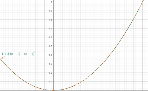$$ g(x) = 1 + 2 \cdot (x - 1) + (x - 1)^2 \quad \text{and} \quad f(x) = x^2 $$

Taylor Figure 1. Taylor Approximation

As you can see, the two functions behave similarly near $x_0 = 1$, so $g(x)$ correctly approximates $f(x)$ in that region.

The more terms (thus more derivatives) we consider in the Taylor series, the better the approximation. But for our purposes, we’re happy stopping at the first derivative:

$$ f(x) \approx f(x_0) + f'(x_0) \cdot (x-x_0) $$

This formula tells us how the function locally behaves. The first derivative $f'(x_0)$ tells us the speed and direction of increase, while $(x - x_0)$ represents a step from the starting point.
But remember: our goal is to minimize. We don’t want to go toward growth, but in the opposite direction, and we want to do it with a small step, chosen arbitrarily. So we write the step as:

$$ x - x_0 = -\eta \cdot f'(x_0) $$

where:

$\eta$ is the step size
$-f'(x_0)$ is the opposite direction of increase

So we have:

$$ x = x_0 - \eta \cdot f'(x_0) $$

Sound familiar?

Going back, if we substitute this into Taylor's formula, we get:

$$ f(x_0 - \eta \cdot f'(x_0)) \approx f(x_0) - \eta \cdot f'(x_0)^2 $$

Let’s simplify the notation:

$$ x_0 = x_t $$

and

$$ x_t - \eta \cdot f'(x_t) = x_{t+1} $$

where:

$x_t$ is the starting point
$x_{t+1}$ is the next point

So:

$$ f(x_{t+1}) \approx f(x_t) - \eta \cdot f'(x_t)^2 $$

Now suppose $f$ is a Convex Function and Lipschitz Continuous, we can then assert this inequality:

$$ f(x_{t+1}) \leq f(x_t) - \frac{\eta}{2} \cdot f'(x_t)^2 $$

with

$$ 0 < \eta \leq \frac{1}{L} $$

where $L$ is a Lipschitz constant.

In words: the function $f$, when moving from $x_t$ to $x_{t+1}$, decreases, as long as we choose $\eta$ small enough. And that’s exactly what we wanted!
With the rule

$$ x = x_0 - \eta \cdot f'(x_0) $$

the function decreases with each step.

So, if $f$ is the loss function and $x$ is some generic weight,
we’ve just derived the formula for gradient descent.

This was meant to give a "simple" intuition. If you're looking for a formal, rigorous proof, I recommend this source.

About Activation Functions

In this section we finally answer why the Heaviside Step was ruthlessly discarded as an activation function. If you’ve read the whole article, you’ve seen that backpropagation requires this computation:

$$ \frac{\partial L }{\partial w_i} = \frac{\partial L(\sigma(H(x_i, w_i))) }{\partial w_i} = \frac{\partial L }{\partial p} \cdot \frac{\partial p }{\partial net} \cdot \frac{\partial net }{\partial w_i} $$

where:

$\frac{\partial p }{\partial net}$ is the derivative of the activation function with respect to the transfer-function output.
$\frac{\partial L }{\partial p}$ is the derivative of the loss with respect to the prediction.

To compute these derivatives, both the loss $L$ and the activation $\sigma$ must be differentiable. The trouble is that the Heaviside step has a discontinuity at $x = 0$, so it’s not classically differentiable. (Strictly speaking it is differentiable in the theory of distributions: its derivative is the Dirac Delta.) But that derivative isn’t something we can drop directly into our algorithm. Notice that ReLU is also non-differentiable at $x = 0$, yet no one rejects it for that reason. In the image below, you can see how it behaves:

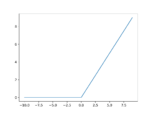ReLU Figure 2. ReLU

So why all the hostility toward Heaviside?

Although ReLU is non-differentiable at $x = 0$, it is continuous there, so we can assign an artificial sub-gradient between 0 and 1: the function is sub-differentiable. With Heaviside that’s impossible. And even if (for argument’s sake) we chose to use the Dirac Delta as its derivative... look here:

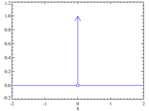Figure 3. Dirac Delta

As you can see, it is zero everywhere except at $x = 0$.
That means the gradient would be always zero, the weights would never change, and the neural network would learn nothing.
Finally, there’s a secondary snag: Binary Cross-Entropy blows up to infinity if the prediction is exactly 0 or 1. The sigmoid avoids that because it only reaches those values asymptotically.

From One to Many

This last section gives a general idea of why we need networks with many neurons.
We’ve seen that a single perceptron can reach a solution, it eventually separates the AND problem correctly. So why add complexity?
First examine the transfer function. For the two-dimensional AND problem we have

$$ net = w_1 \cdot x_1 + w_2 \cdot x_2 + b $$

For some of you, this formula won’t mean much. For others, it may dredge up bad memories of the line equation in its implicit form. Back-propagation is finding the line’s coefficients so that we can do this:

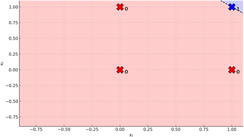Line AND Figure 4. Line on the AND Problem

That is, separate the 0-cases from the 1-cases. If you can do that, the data are linearly separable, and one perceptron suffices.
Now look at the XOR problem. It’s a logical operation like the AND problem, but it has a different truth table:

$$ \begin{array}{|r|r|r|} \hline x_1 & x_2 & XOR(x_1,x_2)\\ \hline 0 & 0 & 0\\ \hline 0 & 1 & 1\\ \hline 1 & 0 & 1\\ \hline 1 & 1 & 0\\ \hline \end{array} $$

Let’s see what happens geometrically:

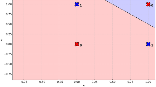Line XOR Figure 5. Line on the XOR Problem

You can bang your head and swear all you like, but you’ll never find a single straight line that separates the 0s from the 1s. It’s impossible. That’s exactly why the XOR problem is said to be not linearly separable. If only we could add another line, then we really could do this:

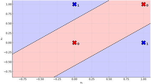Boundary XOR Figure 6. Two Lines on the XOR Problem

But wait a second... who’s to say we can't? After all, one neuron gives you one line, so two neurons give you two lines, right? And there we have it: a clear reason why we need more neurons. But how much does that change everything we’ve seen so far!? Before we answer, let’s see what our neural network now looks like:

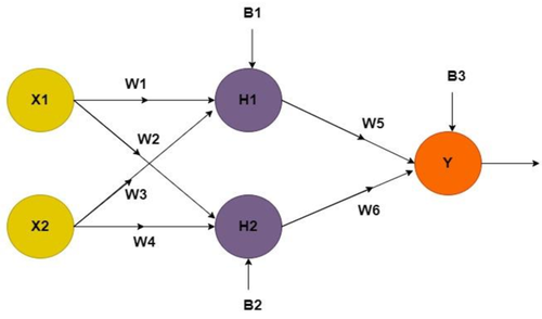NN XOR Figure 7. Neural Network for XOR Problem

If you’re thinking, "Come on Luca, you said one extra neuron was enough! I’m outraged!1!!" well, yes, that’s still true. But classic feed-forward networks insist that the number of input neurons matches the number of features, so you’re stuck with this setup. Maybe one day I’ll tell you the incredible story of neuroevolution, where things get very different. But back to us...
Everything else actually stays the same; the only twist is that we have to dig deeper into the equation for the derivative of the error with respect to a weight, because now the output of one neuron becomes the input of the next. Focusing on neurons $Y$ and $H_1$, the output of $H_1$ is:

$$ h_1 = \sigma_{H_1}(net_{H_1}) = \sigma(w_1 \cdot x_1 + b_1) $$

and $Y$'s output is:

$$ \sigma_Y(net_Y) = \sigma\!\bigl(w_5 \cdot \sigma_{H_1}(net_{H_1}) + b_3\bigr) = \sigma\!\bigl(w_5 \cdot \sigma(w_1 \cdot x_1 + b_1) + b_3\bigr) $$

Rewriting it in a form we’ve already used, we get:

$$ \frac{\partial L}{\partial w_5} = \frac{\partial L}{\partial p} \cdot \frac{\partial p}{\partial net_Y} \cdot \frac{\partial net_Y}{\partial w_5} $$

$$ \frac{\partial L}{\partial w_1} = \frac{\partial L}{\partial p} \cdot \frac{\partial p}{\partial net_Y} \cdot \left( \frac{\partial net_Y}{\partial h_1} \cdot \frac{\partial h_1}{\partial net_{H_1}} \cdot \frac{\partial net_{H_1}}{\partial w_1}\right) $$

where:

$\frac{\partial net_Y}{\partial h_1}$ is the derivative of $Y$'s transfer function with respect to $H_1$'s activation function
$\frac{\partial h_1}{\partial net_{H_1}}$ is the derivative of $H_1$'s activation function with respect to its transfer function
$\frac{\partial net_{H_1}}{\partial w_1}$ is the derivative of $H_1$'s transfer function with respect to the weight $w_1$

And I’d say, for the sake of our sanity, we can stop here, but the very same reasoning applies to:

$$ \frac{\partial L}{\partial w_2} \quad \text{and} \quad \frac{\partial L}{\partial w_6}. $$

With $n$ neurons you have $n$ lines (or segments) forming a piece-wise curve that separates data that are not linearly separable, In short... it can effortlessly pull off this monstrosity.

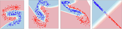n-segment Boundary Figure 8. Network Decision Boundary with Many Neurons

One last note before we get to the conclusions. For simplicity, we focused on the two-dimensional case and therefore talked about lines, but the same reasoning holds in higher-dimensional spaces. There, we speak of hyperplanes instead of lines.

To Wrap Up

Alright folks, we’ve reached the end of our series of articles on the neuron. And to borrow a famous quote:

Here comes the end of our fellowship... I will not say do not weep, for not all tears are an evil.

Obviously I'm talking about the fellowship of neuron, because more articles are on the way. In life, only a few things are certain: death, taxes, and another one of my articles. I hope you enjoyed this series as much as I enjoyed writing it.

Until next time.

Neurons for Dummies - 3

The Chain Rule

Gradient Descent

About Activation Functions

From One to Many

To Wrap Up

Related Posts

Published

Category

Tags

Contacts