

The holidays have just passed. And yes, I know it is February, but the writing of this article started on January 5, so nothing, the holidays have just passed. All of us have had lunches, dinners, and little dinners, and I am sure you have been harassed by the usual generic political discussions made by the blue collar relative (worker but doctor in his free time) who knows that vaccines cause autism. Because he informed himself. I can already imagine it, I can already hear it echoing inside me
Chernobyl also did some good things...
Ah no, wait a moment, that was not exactly the sentence. Alright then let's start again, this time less paraphrased... what did Chernobyl leave us!? And before you ask, I mean beyond the widespread ignorance and the ancestral fear of nuclear energy (if it was not clear I am a supporter of atomic energy). Well yes, it left us a beautiful optimization algorithm. And since I am a big fan of everything that is weird, I decided to talk about it. So everyone grab your lead jackets and let's begin.
3, 2, 1... Ignition
Ignition means startup, but what is starting up is not an engine, it is a reactor. Now, I am not saying that we should thank Dyatlov for his terrible job, but thanks to his terrible job this algorithm came out. Sure, I am clearly seeing the glass half full, but we are dancing now, so let's dance.
Let's start by saying that it is a physics-inspired algorithm, and like any good metaheuristic algorithm, its goal is the search for the optimum, and we will get to what that means. Now, far be it from me to explain the physics of particles, also because I do not know it and honestly studying it to write an article about a metaheuristic algorithm seems a bit overkill. In any case, when a nuclear power plant explodes, among the various isotopes and particles emitted by the unstable core, there are the three protagonists of our story, which are alpha particles, beta particles, and gamma rays.
- Alpha particles are the big boned ones, and therefore more "slow". Think that they reach only about \(\sim 5 \%\) of the speed of light, poor losers. In any case they are composed of two protons and two neutrons. They therefore have a positive charge which in matter is very high, and precisely for this reason they are strongly ionizing (for the record, ionizing \(\rightarrow\) molecular destruction \(\rightarrow\) radiation poisoning \(\rightarrow\) you melt \(\rightarrow\) you die). The fact that they are very bulky, however, also makes them poorly penetrating. To be clear, if you are behind a sheet of paper you are safe, at least until you breathe them in and or ingest them, in that case it has been nice and we will see each other on the other side of the Styx.
- Beta particles have followed the ketogenic diet and are a little more slim: they reach about \(\sim 30–90 \%\) of the speed of light. Their mass is small, since they are composed of an electron, and they have a negative charge. They are a bit more insidious than alpha particles, especially from the outside, but they can be easily shielded with a few millimeters of metal such as aluminum. If you are not behind shielding, however, tough luck. They are less ionizing than alpha particles, but since they are often very energetic, the interaction with the atoms of our body makes the orbiting electrons fly away (and here comes back the molecular destruction).
- Gamma rays are electromagnetic waves. They are made of photons (you know, the ones responsible for light transmission) and therefore have no mass.
Basically they are the Ariana Grande of particles and travel at the speed of light. Unless you have raised a
lead wall Fortnite style, they have a very high penetrating power. Their danger derives from how they interact with matter. They can do so in three ways:
- Photoelectric effect: All the energy of the photon is transferred to an electron of the atom which is ejected from its orbit.
- Compton effect: The photon gives up part of its energy resulting in a free and very angry electron.
- Pair effect: Part of the energy is converted into mass creating an electron and a positron which interact with other electrons like beta particles.
What happens if you get hit by gamma rays?! If you are lucky you become the incredible Hulk, if you are unlucky (and you will be unlucky), you fall into the previous cases and goodbye.
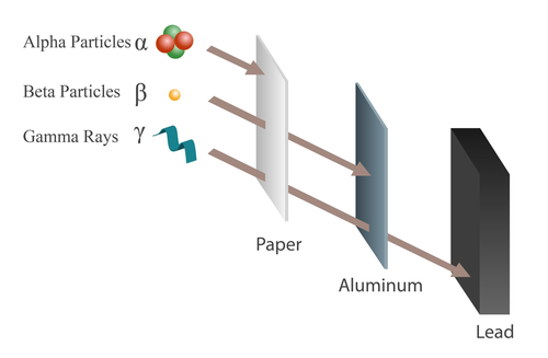 Figure 1. Alpha and Beta particles, Gamma rays
Let's conclude this paragraph with a question (and also an answer). If unfortunately a power plant were to explode, what is the first thing people do? Exactly, they run away. They try to get to safety to escape all the bad things presented. After all, who wants to become a big green and angry brute?
Radiation, Panic, and Local Minima
We stopped, in the previous paragraph, with people running away screaming. Now I do not want to say that ionizing radiation, like bloodhounds, goes looking for people, but in this algorithm people actually represent the objective. A person runs away from the explosion point, and our friends go in search of them, which corresponds to the search for the optimum. Macabre? Yes. Not very realistic? Also. But come on, it is awesome (maybe for the citizens of Pripyat it is a bit less so). This is what it means to search for the optimum in the Chernobyl Disaster Optimizer (CDO). As for how, well... keep reading.
We have identified the four elements necessary for the CDO. Let's see how they are used algorithmically.
The Human
The human, our sacrificial victim. The poor man future Hulk. As we said, he runs away, and intuitively the farther he gets the more safe he feels, until he stops. This is modeled through the following formula:
Formula 1. Speed Decay
That is, the escape speed is initially maximum, \(3mph\) (yes, the author uses miles per hour as the unit), and as the iterative algorithm progresses, the speed decreases until it reaches zero. In the formula:
- \(it\) is the current iteration
- \(n_{it}\) is the number of iterations that will be performed by the algorithm.
As will be seen from the following formulas, the particles do not see the man and do not know where he is, but they are rewarded when they get closer to him. Whoever gets closest becomes a guide for the others.
Particles and Rays
Our ambassadors that bring pain: the particles of the algorithm. They start from the explosion point in search of the man to irradiate. Like many metaheuristic algorithms, CDO is population based. This means that we have a family of particles where each particle is a list with size equal to the dimensionality of the problem to be solved, and represents a possible solution to the problem itself. Each of them is associated with a fitness which is used to determine how good a particle is at solving a problem. The higher or lower the fitness (depending on the type of problem, whether maximization or minimization), the closer it gets to the optimal solution in the search space. Let's see how, mathematically, they move to find their target. In my implementation, all particles have random positions, and the best ones (or leaders) are initially placed at the origin, which in the metaphor coincides with the explosion point.
def _update_best_particles(self, fitness: float, pos: np.ndarray, alpha_score: float, alpha_pos: np.ndarray,
                           beta_score: float, beta_pos: np.ndarray, gamma_score: float, gamma_pos: np.ndarray):
  is_alpha_better = self._is_better(fitness, alpha_score)
  is_beta_better = self._is_better(fitness, beta_score)
  is_gamma_better = self._is_better(fitness, gamma_score)

  if is_alpha_better is True:
      alpha_score, alpha_pos = fitness, pos.copy()

  if is_alpha_better is False and is_beta_better is True:
      beta_score, beta_pos = fitness, pos.copy()

  if  is_alpha_better is False and is_beta_better is False and is_gamma_better is True:
      gamma_score, gamma_pos = fitness, pos.copy()

  return alpha_score, alpha_pos, beta_score, beta_pos, gamma_score, gamma_pos

def optimize(self):
  alpha_pos = np.zeros(self._dim)
  beta_pos = np.zeros(self._dim)
  gamma_pos = np.zeros(self._dim)
  alpha_score = np.inf if self._approach == "min" else -np.inf
  beta_score = np.inf if self._approach == "min" else -np.inf
  gamma_score = np.inf if self._approach == "min" else -np.inf

  ...

  for it in range(self._n_iter):
      for particle_i in range(self._n_particles):
          current_particle = self._clip(particles[particle_i])
          particles[particle_i] = current_particle
          fitness = float(self._function_to_optimize(current_particle))

          (alpha_score, alpha_pos, beta_score,
           beta_pos, gamma_score, gamma_pos) = \
            self._update_best_particles(fitness, current_particle, alpha_score, alpha_pos,
                                        beta_score, beta_pos, gamma_score, gamma_pos)
      ...
Snippet 1. Definition of the Leaders
As can be seen from Snippet 1 only the three alpha, beta, and gamma leaders are extracted, that is the best solutions found up to that moment.
This is because the best ones are those closest to the optimal solution (the man), and they are good candidates to guide
the exploration of the search space of the others, in a given iteration. Moreover, the update of the particles happens with strict criteria as can be seen
from the _update_best_particles function. This allows avoiding continuous changes and therefore having a controlled evolution
of the particle positions, favoring the convergence of the solution.
Up to this point it is fairly clear, right? Random particles, fitness, best ones that emerge. Now comes the interesting part: how the hell do we make them move?
Now a few formulas begin. For each particle \(\xi\), or rather for each component \(col\) of each particle \(\xi\), we compute what the author calls the Gradient Descent Factor. Do not be misled by the name though, this is not a gradient since no derivative appears. It is instead a coefficient that indicates how strongly a component is pushed toward one of the leader particles (alpha, beta, or gamma), which at that moment represent the best solutions found. In formulas we have:
Formula 2. Gradient Descent
Alright, that is a lot of symbols. But let's go in order. First of all, I start by saying that the \(p\) in the subscript is used to indicate the reference leader, so \(p=\alpha, \, \beta, \, \gamma\). This is because the formulas change depending on the leader considered, starting from the quantity \(\varphi_{p}\) which can be interpreted as a scaling factor:
Formula 3. Scaling Factors
As for the term \(POS_{p}^{col}\), it simply represents the position component of the leader particle. In fact, we said that each particle is a list, and that \(col\) is used to indicate the i-th element of the list. To avoid any confusion, if we considered a two-dimensional optimization problem, Formula 2 would be executed six times for each particle. This is because it is executed once for each element of the list, and for each element the leader \(\alpha\) is considered first, then \(\beta\), and finally \(\gamma\).
Let's move on to the next term, \(PROP_{p}\). We can see it as an area of influence: the larger this area is, the more particles fall under the effect of the leader and therefore tend to follow it, that is their movement is computed with respect to this region. It is defined as follows:
Formula 4. Propagation Factors
In this formula we see old and new friends. We have already introduced \(\varphi_{p}\) and \(WS\). There is no need to tell you what \(\pi\) is. Instead, \(r_{1, \, p}^2\) is a random numerical value between \(0\) and \(1\) (the subscript \(p\) is used to indicate that each leader will have its own random radius), \(rand_p \left( 0, \, 1 \right)\) is exactly the same thing. Much more interesting, instead, is \(\upsilon_{p}\). This represents a velocity associated with the leader and is a function of the leader considered. It is defined as follows:
Formula 5. Leader Velocities
If you remember, in the previous paragraphs I had talked about how fast the particles were. Well, that discussion was necessary precisely to get to this point. Each leader has its own velocity defined as the base \(10\) logarithm of a random number taken between \(1\) and the maximum speed for that type of particle. The use of the logarithm serves to reduce potentially very large values, avoiding instability of the algorithm.
We are almost there, one last ingredient is missing. \(D_{p}\) represents the distance between the current particle \(\xi\) and the effect of the leader \(p\), taking into account its propagation. It is defined as follows:
Formula 6. Distance
In this formula we have \(A_{p}\) which is the propagation area associated with the leader \(p\) and is a measure of the extension of its search space. Similarly to before, it is computed as follows:
Formula 7. Propagation Area
And \(\xi_i^{col}\) and \(POS_{p}^{col}\), which have already been introduced. Since repetita iuvant, \(\xi_i^{col}\) is the value contained in the position \(col\) of the i-th particle (not to be confused with the leader), and \(POS_{p}^{col}\) is the value contained in the position \(col\) of the leader particle \(p\).
Alright, I was joking, it was not really the last ingredient. But now that we have defined all the necessary formulas we can compute \(GDF_{p}\) and therefore proceed with the calculation of the new value of the position components of each particle. So we update the value of \(\xi_i^{col}\) in the following way:
Formula 8. Position Component Update
Yes, there are a lot of formulas, but I swear they are finished. So here is a code snippet that implements what has been written:
def optimize(self):

  ...

  new_positions = np.empty_like(particles)

  for particle_i in range(self._n_particles):
    for particle_col in range(self._dim):
      particle_col_val = particles[particle_i, particle_col]

      r1 = self._np.random()
      r2 = self._np.random()
      alpha_prop = (np.pi * r1 * r1) / (0.25 * speed_alpha) - walking_speed * self._np.random()
      alpha_prop_area = (r2 * r2) * np.pi
      alpha_col_val = alpha_pos[particle_col]
      D_alpha = abs(alpha_prop_area * alpha_col_val - particle_col_val)
      gdf_alpha = 0.25 * (alpha_col_val - alpha_prop * D_alpha)

      r1 = self._np.random()
      r2 = self._np.random()
      beta_prop = (np.pi * r1 * r1) / (0.5 * speed_beta) - walking_speed * self._np.random()
      beta_prop_area = (r2 * r2) * np.pi
      beta_col_val = beta_pos[particle_col]
      D_beta = abs(beta_prop_area * beta_col_val - particle_col_val)
      gdf_beta = 0.5 * (beta_col_val - beta_prop * D_beta)

      r1 = self._np.random()
      r2 = self._np.random()
      gamma_prop = (np.pi * r1 * r1) / speed_gamma - walking_speed * self._np.random()
      gamma_prop_area = (r2 * r2) * np.pi
      gamma_col_val = gamma_pos[particle_col]
      D_gamma = abs(gamma_prop_area * gamma_col_val - particle_col_val)
      gdf_gamma = gamma_col_val - gamma_prop * D_gamma

      new_positions[particle_i, particle_col] = (gdf_alpha + gdf_beta + gdf_gamma) / 3.0

  ...
Snippet 2. Particle Update
I would like to conclude this paragraph with a note. Any good metaheuristic algorithm faces the problem of exploration vs exploitation, that is continuing the search at a global level while at the same time continuing to exploit the good solutions found so far. In this algorithm this is done through the leaders and their propagation areas. In fact, if you remember well, the alpha leader does not go very far since it is easily shielded and has reduced speed. This is what also happens in the algorithm. The alpha leader encourages a local search and therefore the exploitation of the good solutions already known. Through its propagation area, the search is carried out in its local neighborhood. On the other hand, beta and gamma, thanks to higher speed and propagation explore regions farther away in the search space, previously unknown.
At the end of the algorithm, the best solution (which I remind you is the particle with the highest or lowest fitness) is given by the alpha leader.
The Explosion
How is this algorithm triggered?! Well, simply by instantiating and calling the class defined by me:
function = lambda x: np.sin(x[0]) * (np.exp(1-np.cos(x[1])) ** 2) + np.cos(x[1]) * (np.exp(1-np.sin(x[0])) ** 2) + (x[0]-x[1]) ** 2

cdo = CDO(n_particles=30, dim=2,
          approach='min', n_iter=20,
          bounds=(-2 * np.pi, 2 * np.pi), function_to_optimize=function)

best_fitness, best_particle, _ = cdo.optimize()

print(f'Best Fitness is {best_fitness} with Particle {best_particle}')
Snippet 3. Algorithm Usage
It is worth spending a couple of words on the constructor arguments.
n_particlesindicates the number of particles you want in your particle population. Generally, the higher it is, the greater the probability of reaching the optimum, but it results in a slowdown of the algorithm.function_to_optimizeanddimare the mathematical function to optimize, and its dimensionality. In my specific case I used the Bird Function, which has dimension \(2\) and is known for the difficulty of computing its minimum.approachindicates whether you want to minimize (min) or maximize (max).boundsindicates the existence limits of the function. It is useful when we know that we need to search for the optimum in a specific portion of the domain.
By running this snippet you should get an output similar to:
Best Fitness is -106.3248972989146 with Particle [4.74192243 3.21810325]
where the values contained inside the particle are the coordinates \((x, \, y)\) that get very close to the minimum of the function, within the given domain. Worth noting is the use of the word "should", since this is a probabilistic process.
To Wrap Up
I have to say that I really like these exotic algorithms and it was fun to study and implement it. But this is with hindsight. The original paper in fact is not only written rather poorly but also contains several inaccuracies in the formulas. For this reason, in writing this article I relied partly on that, partly on a more recent second paper and on the Matlab code provided by the author of the algorithm. What came out is, in fact, a work of reverse engineering and reconstruction of information, necessary to give a coherent and usable form to the algorithm. As always, I leave you the link to my implementation so that you can take a look at the code and run your experiments. Watch out for radiation.
Until next time.