Not Only BackProp

Do you ever wake up in the morning thinking:
Damn, today I really feel like backpropagating some error... but I should probably watch my weight! No? Weird, but hey, good for you. Either way, even if nobody asked, I’ve got the perfect solution: the right compromise between indulgence and good taste. Jokes aside, this article is more of a conceptual exercise. Dedicated to those who, like me, believe houses are meant to be lived in and whose social battery hits 0% after 8:00 PM. Today, I’ll talk about how I used the Crystal algorithm instead of backpropagation to tweak and thus, train a neural network. Never heard of Crystal? Tsk tsk, shame on you. That means you haven’t read my article about it. But don’t worry, you can catch up here. And if you’re also missing the legendary backpropagation, no panic: you’ll find the whole neuron saga here.

But Why!?

If that’s your question, well I already told you that the asociality-after-8PM combo leads to weird ideas. Why on earth would anyone want to train a neural network without backpropagation, which already works so well...?
You really want the answer...?
Because I can.
Jokes aside, it’s not as far-fetched as it sounds. Let’s take a moment to reconsider the limitations of backpropagation:

• It requires both the loss and activation functions to be differentiable.
• It only looks at the local shape of the error function, not the global one. This can lead to local minima, where you think you’ve found a low error value but, really, you’re just unable to see beyond your own nose.
• Overfitting: that wonderful moment when you overtrained the network and it stops generalizing. It knows the training data too well, but has no clue what to do with anything new. Think of it like this: it’s one thing to teach you how addition works (generalization), and another to teach you only that 2+2 (memorization).
• Vanishing/Exploding Gradient: Gradients can:
  • Become zero. When that happens, weights stop changing and the network stops learning.
  • Become too large. Then, the weights explode and the network becomes hypersensitive to inputs, a tiny variation at the input sends the output into a meltdown.

But enough with the badmouthing of backpropagation, if you’ve got something to say, say it to its face if you dare. Still, why do we keep using it despite all these limitations? Well, because for each of those problems, there’s a workaround. Except for differentiability, no escaping that one. But let’s dig in our heels and take a look at an alternative. Why might using a metaheuristic, and in this case, the Crystal algorithm, actually overcome those limitations? Let’s break it down:

• When using a metaheuristic algorithm, you don’t need to compute derivatives. So you can use whatever loss (and activation) function your heart desires. Even the one your uncle’s cousin’s Facebook friend swears the government tried to suppress. And yes, you can totally use the Heaviside step function.
• The process of modifying weights is fundamentally different from backpropagation. Remember the hiker slowly descending the loss mountain step by step? Well, that metaphor is obsolete here. Weight updates aim to minimize the loss globally, not just locally, so the risk of getting stuck in a "valley" (aka local minimum) is greatly reduced.
• Since it's a probabilistic process, there’s a lower chance of the model overfitting to the data, making the solution more robust.
• And since there's no more gradient descent... well, there’s no gradient at all. Goodbye vanishing and exploding gradients.

But, like every good story, this one comes with its own set of issues. I know, size doesn’t matter but for these algorithms, it actually does. If the network is too large, this approach becomes simply impractical, and in general, it's less efficient than backpropagation. It might also take longer to reach convergence, that is to find a set of weights that make the network perform well. So, when should you use one over the other?
As with most things in life: it depends. In general, a metaheuristic approach can be useful when dealing with very noisy data, or when the risk of overfitting is particularly high. In such cases, it may be worth testing the network’s performance with an alternative method, like Crystal. That said, backpropagation remains the default choice in most cases. It’s far more computationally efficient, and many of its shortcomings can be mitigated with the right techniques and, something far too often overlooked, with proper data cleaning.

But How!?

The Data

In this section, we’ll see how the experiment was carried out at the code level. Rule number one of deep learning: never talk abou...oh wait, wrong script! The data, right. For the dataset, I used the legendary Iris dataset, consisting of 150 samples with 4 features each, used to classify 3 species of iris flowers:

• Iris Setosa
• Iris Virginica
• Iris Versicolor

If flowers make you gag, feel free to skip ahead. Otherwise, here’s what the features look like:

• Sepal length (cm): Length of the sepalo
• Sepal width (cm): Width of the sepal
• Petal length (cm): Length of the petal
• Petal width (cm): Width of the petal

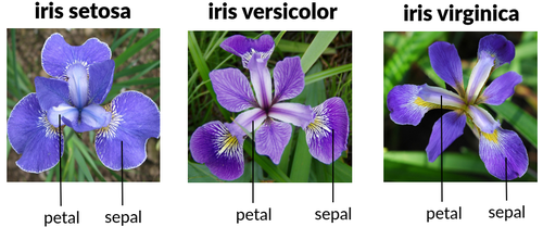Figure 1. Iris Features

Sometimes you might come across a fifth column: id. Spoiler alert: it’s completely useless. It’s just a unique identifier, so it always gets discarded because it doesn’t provide any meaningful information. The goal of the neural network is pretty straightforward on paper: guess which type of Iris we’re looking at, based on the numeric values of the 4 features.
This is considered an entry-level problem in the deep learning world, but don’t be fooled: if someone handed you just the numbers, you wouldn’t have the slightest clue what’s going on (sticking with the botanical theme here, you’d be as lost as a chickpea in a tulip field).

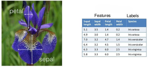Figura 2. Iris Classification

The Network

Since I wanted to compare the training performance of backpropagation and Crystal, I started off nice and simple by creating two identical neural networks using the PyTorch framework.
Let’s begin with the definition of the neural network:

class SimpleNet(nn.Module):

    def __init__(self):
        super().__init__()
        self.net = nn.Sequential(
            nn.Linear(4, 16),
            nn.ReLU(),
            nn.Linear(16, 3)
        )

    def forward(self, x):
        return self.net(x)

The architecture is very simple. And trust me, if this looks complicated to you... it’s only because you haven’t seen anything yet.
This network includes:

• 4 input neurons
• 16 neurons in a single hidden layer
• 3 output neurons

Graphically, we could represent it like this:

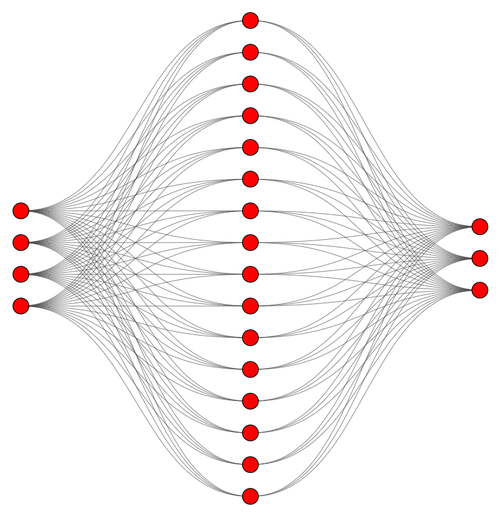Figura 3. Neural Network Architecture

These numbers weren’t just picked at random well, except for the 16, which you can absolutely tweak depending on your mood, planetary alignment, or how much coffee you’ve had.

• The input layer must have 4 neurons because there are 4 features in the dataset.
• The output layer must have 3 neurons because we’re classifying 3 types of iris.

With some quick math, we can compute the number of parameters in the network:

• Number of weights in the hidden layer:

\(4 \cdot 16 = 64\)

• Number of biases in the hidden layer:

\(16\)

• Number of weights in the output layer:

\(3 \cdot 16 = 48\)

• Number of biases in the output layer:

\(3\)

So, the total number of parameters is:

\(64 + 48 + 16 + 3 = 131\)

And this number is anything but trivial: it will directly determine the crystal size in the Crystal algorithm.
Alright, now that we’ve defined the network, let’s not forget that we want two identical copies and by identical, I mean same architecture and same initial weights. Otherwise... what kind of comparison would that be!?
Now, when you create a network with PyTorch, weights are initialized in a consistent, but still random way. So here’s what I did: I created a third ghost network, whose sole purpose in life is to provide the initial weights. Those weights are then copied into both of the real networks that I’ll be training. Of course, you could also save your own custom weights and reload them whenever you like... but hey, generating them is your responsibility, so don’t come crying later.
Here’s the code:

def create_networks(weights: str = "weights.pth"):
    if os.path.exists(weights):
        print(f"Loading weights from {weights}")
        initial_weights = torch.load(weights)
    else:
        print("Creating and Saving new weights...")
        initial_weights = SimpleNet().state_dict()
        torch.save(initial_weights, weights)

    nn_model_backp = SimpleNet()
    nn_model_crystal = SimpleNet()
    nn_model_backp.load_state_dict(deepcopy(initial_weights))
    nn_model_crystal.load_state_dict(deepcopy(initial_weights))
    return nn_model_backp, nn_model_crystal

If you're wondering why I used deepcopy, I strongly recommend a quick refresher on OOP, especially the concept of encapsulation.
Spoiler: we want to avoid a situation where changing one network also changes the other. You take your eyes off the code for one second and boom, anarchy.

Everything Else

Now that we’ve defined our network, let’s take a look at the rest of the code. Since we don’t like to miss out on anything fancy, the optimizers were implemented using the strategy pattern.
Here are the abstract class and the context class:

class AOptimizer(ABC):

    def __init__(self, nn_model: nn.Module, loss_function):
        self._model = nn_model
        self._loss_function = loss_function

    @property
    def model(self) -> nn.Module:
        return self._model

    @model.setter
    def model(self, nn_model) -> None:
        self._model = nn_model

    @property
    def loss_function(self) -> loss._WeightedLoss:
        return self._loss_function

    @loss_function.setter
    def loss_function(self, loss_function: loss._WeightedLoss) -> None:
        self._loss_function = loss_function

    @abstractmethod
    def optimize(self, X_train: np.ndarray, y_train: np.ndarray) -> None:
        raise NotImplementedError

    @staticmethod
    @abstractmethod
    def get_name() -> str:
        raise NotImplementedError

    def evaluate(self, X_test: np.ndarray, y_test: np.ndarray) -> float:
        X_test = torch.tensor(X_test, dtype=torch.float32)
        y_test = torch.tensor(y_test, dtype=torch.long)
        preds = self._model(X_test).argmax(dim=1)
        acc = (preds == y_test).float().mean()
        return acc

class Optimizer:

    def __init__(self, strategy: AOptimizer = None):
        self._strategy = strategy

    @property
    def strategy(self) -> AOptimizer:
        return self._strategy

    @strategy.setter
    def strategy(self, strategy: AOptimizer) -> None:
        self._strategy = strategy

    def optimize(self, X_train: np.ndarray, y_train: np.ndarray) -> None:
        self._strategy.optimize(X_train, y_train)

    def evaluate(self, X_test: np.ndarray, y_test: np.ndarray) -> float:
        return self._strategy.evaluate(X_test, y_test)

While the concrete strategies are two.
The one that implements backpropagation:

class BackpropOptimizer(AOptimizer):

    def __init__(self, nn_model, loss_function):
        super().__init__(nn_model=nn_model, loss_function=loss_function)

    @staticmethod
    def get_name():
        return "Backprop"

    def optimize(self, X_train: np.ndarray, y_train: np.ndarray) -> None:

        print(f"Start optimization for {BackpropOptimizer.get_name()} Strategy")

        X_train_t = torch.tensor(X_train, dtype=torch.float32)
        y_train_t = torch.tensor(y_train, dtype=torch.long)
        train_loader = DataLoader(TensorDataset(X_train_t, y_train_t), shuffle=False)

        opt = optim.Adam(self._model.parameters(), lr=0.01)
        for epoch in range(21):
            for xb, yb in train_loader:
                opt.zero_grad()
                out = self._model(xb)
                loss = self._loss_function(out, yb)
                loss.backward()
                opt.step()

            if epoch % 10 == 0:
                print(f"Epoch {epoch}, Loss: {loss.item():.4f}")

        acc = self.evaluate(X_test=X_train, y_test=y_train)
        print(f"Accuracy on Train Set: {acc:.2%}")

and the one that implements Crystal:

class CrystalOptimizer(AOptimizer):

    def __init__(self, nn_model, loss_function):
        super().__init__(nn_model=nn_model, loss_function=loss_function)

    ...

    @staticmethod
    def get_name() -> str:
        return "Crystal"

    def _is_new_fitness_better(self, old_crystal_fitness, new_crystal_fitness) -> bool:
        return new_crystal_fitness < old_crystal_fitness

    def _flat_weights(self) -> np.ndarray:
        weights = []
        for p in self._model.parameters():
            weights.append(p.data.view(-1))
        weights = torch.cat(weights).detach().cpu().numpy()
        return weights

    def _create_crystals(self, lb: int, ub: int, nb_crystal: int) -> (np.array, int, int):
        base_weights = self._flat_weights()
        dim = base_weights.size
        random_crystals = np.random.uniform(low=lb, high=ub, size=(nb_crystal - 1, dim))
        crystals = np.vstack([base_weights, random_crystals])
        print(f"Created {crystals.shape[0]} Crystals With {crystals.shape[1]} Elements")
        return crystals

    def _assign_weights(self, crystal: np.ndarray) -> None:
        cum_p = 0
        for p in self._model.parameters():
            total_params = p.numel()
            tensor = torch.tensor(crystal[cumulative_nb_params:cum_p + total_params])
            reshaped_tensor = tensor.view(p.shape)
            p.data.copy_(reshaped_tensor)
            cum_p += total_params

    def _evaluate_crystals(self, crystals: np.ndarray, X_train: torch.Tensor, y_train: torch.Tensor) -> (np.ndarray, float, int):
        losses = []
        for crystal in crystals:
            self._assign_weights(crystal)
            with torch.no_grad():
                outputs = self._model(X_train)
                loss = self._loss_function(outputs, y_train)

            losses.append(loss.item())

        fitnesses = np.array(losses).reshape(-1, 1)
        best_index = np.argmin(fitnesses)
        best_value = fitnesses[best_index, 0]
        return fitnesses, best_value, best_index

    def optimize(self, X_train: np.ndarray, y_train: np.ndarray) -> None:
        print(f"Start optimization for {CrystalOptimizer.get_name()} Strategy")

        X_train_t = torch.tensor(X_train, dtype=torch.float32)
        y_train_t = torch.tensor(y_train, dtype=torch.long)

        lower_bound, upper_bound = -2, 2
        nb_crystal = 15
        nb_iterations = 60
        crystals = self._create_crystals(lb=lower_bound, ub=upper_bound, nb_crystal=nb_crystal)
        fitnesses, best_fitness, best_index = self._evaluate_crystals(crystals=crystals, X_train=X_train_t, y_train=y_train_t)
        Cr_b = crystals[best_index]
        for i in range(0, nb_iterations):
            for crystal_idx in range(0, nb_crystal):
                new_crystals = np.array([])
                Cr_main = self._take_random_crystals(crystals=crystals, nb_random_crystals_to_take=1, nb_crystal=nb_crystal).flatten()
                Cr_old = crystals[crystal_idx]
                Fc = self._take_random_crystals(crystals=crystals, nb_crystal=nb_crystal).mean(axis=0)
                r, r_1, r_2, r_3 = self.__compute_r_values()
                Cr_new = self._compute_simple_cubicle(Cr_old=Cr_old, Cr_main=Cr_main, r=r)
                new_crystals = np.hstack((new_crystals, Cr_new))
                Cr_new = self._compute_cubicle_with_best_crystals(Cr_old=Cr_old, Cr_main=Cr_main, Cr_b=Cr_b, r_1=r_1, r_2=r_2)
                new_crystals = np.vstack((new_crystals, Cr_new))
                Cr_new = self._compute_cubicle_with_mean_crystals(Cr_old=Cr_old, Cr_main=Cr_main, Fc=Fc, r_1=r_1, r_2=r_2)
                new_crystals = np.vstack((new_crystals, Cr_new))
                Cr_new = self._compute_cubicle_with_best_and_mean_crystals(Cr_old=Cr_old, Cr_main=Cr_main, Cr_b=Cr_b, Fc=Fc, r_1=r_1, r_2=r_2, r_3=r_3)
                new_crystals = np.vstack((new_crystals, Cr_new))
                new_crystals = np.clip(new_crystals, a_min=lower_bound, a_max=upper_bound)
                new_crystal_fitnesses, new_crystal_best_fitness, new_crystal_best_index = self._evaluate_crystals(crystals=new_crystals, X_train=X_train_t, y_train=y_train_t)
                current_crystal_fitness = fitnesses[crystal_idx][0]
                if self._is_new_fitness_better(old_crystal_fitness=current_crystal_fitness, new_crystal_fitness=new_crystal_best_fitness):
                    crystals[crystal_idx] = new_crystals[new_crystal_best_index]

            fitnesses, best_fitness, best_index = self._evaluate_crystals(crystals=crystals, X_train=X_train_t, y_train=y_train_t)
            Cr_b = crystals[best_index]
            if i % 10 == 0:
                print(f"Iter {i}. Current Best Crystal Fitness Is {best_fitness}")
            self._assign_weights(crystal=Cr_b)
        acc = self.evaluate(X_test=X_train, y_test=y_train)
        print(f"Accuracy on Train Set: {acc:.2%}")

I won’t go into detail about the backpropagation class. All you need to know is that it uses PyTorch, which gives us a high level of abstraction and saves us from going completely insane.
But Luca, I want to know how it actually works!
If you asked yourself that, it means you haven’t read the neuron article series, so GO READ THEM. Instead, let’s focus on the class for the Crystal algorithm. Even here, I’ll only walk through select parts of the code, and you know why? Because I already explained it in a dedicated article. So yes, once again, it’s your fault. Go read that too.
But enough scolding, let’s begin by seeing how the initial population of raw crystals is created. If we printed the network’s structure using this snippet:

from SimpleNet import SimpleNet

net = SimpleNet()
for name, p in net.named_parameters():
    print(name, "|", p.shape)

we’d get the following output:

net.0.weight | torch.Size([16, 4])
net.0.bias | torch.Size([16])
net.2.weight | torch.Size([3, 16])
net.2.bias | torch.Size([3])

What are we actually looking at here? A sequence of matrices and vectors.

• The first item (net.0.weight) is a weight matrix with 16 rows (one for each neuron) and 4 columns (one for each feature). How do I know it’s weights? It literally says so, right there on the left.
• Next comes a bias vector (net.0.bias) with 16 elements, one per neuron. How do I know it’s biases? Again, it says so on the left.

The same goes for the other two lines.
There’s just one small issue: crystals are simple lists of float, while the neural network expects matrices and vectors. So we need to adapt our parameter sequence.
Let’s look at this snippet:

    def _flat_weights(self) -> np.ndarray:
        weights = []
        for p in self._model.parameters():
            weights.append(p.data.view(-1))
        weights = torch.cat(weights).detach().cpu().numpy()
        return weights

    def _create_crystals(self, lb: int, ub: int, nb_crystal: int) -> np.array:
        base_weights = self._flat_weights()
        dim = base_weights.size
        random_crystals = np.random.uniform(low=lb, high=ub, size=(nb_crystal - 1, dim))
        crystals = np.vstack([base_weights, random_crystals])
        print(f"Created {crystals.shape[0]} Crystals With {crystals.shape[1]} Elements")
        return crystals

    def optimize(self, X_train: np.ndarray, y_train: np.ndarray) -> None:
        ...
        nb_crystal = 15
        lower_bound, upper_bound = -2, 2
        crystals = self._create_crystals(lb=lower_bound, ub=upper_bound, nb_crystal=nb_crystal)

What are we doing here?

• With _flat_weights, we iterate over all the network’s parameters, that is the weight and bias matrices and vectors. Each of these structures is flattened into a list. We lose the structure, but keep the content. All of these vectors are then concatenated into one big list of 131 elements (in our case), representing all the weights and biases in the network.
• This list becomes the first crystal of the network, and is used by the _create_crystals function to generate the others randomly, but with the same length. The output is a matrix where each row, that is each crystal, is a complete set of the network’s parameters.

• The parameters lower_bound, upper_bound = -2, 2 and nb_crystal = 15 define:

  • the min and max values that the weights can take
  • the number of crystals to generate

So, we end up with a population of 15 crystals, each with 131 elements ranging from -2 to 2. These values are hyperparameters. How were they chosen? Pure gut feeling. In general: fewer individuals = faster algorithm. Also, we don’t want a network with huge weights, or it’ll become way too sensitive to inputs.
Now let’s move on to another essential snippet:

    def _assign_weights(self, crystal: np.ndarray) -> None:
        cum_p = 0
        for p in self._model.parameters():
            total_params = p.numel()
            tensor = torch.tensor(crystal[cum_p:cum_p + total_params])
            reshaped_tensor = tensor.view(p.shape)
            p.data.copy_(reshaped_tensor)
            cum_p += total_params

    def _evaluate_crystals(self, crystals: np.ndarray, X_train: torch.Tensor, y_train: torch.Tensor) -> (np.ndarray, float, int):
        losses = []
        for crystal in crystals:
            self._assign_weights(crystal)
            with torch.no_grad():
                outputs = self._model(X_train)
                loss = self._loss_function(outputs, y_train)

            losses.append(loss.item())

        fitnesses = np.array(losses).reshape(-1, 1)
        best_index = np.argmin(fitnesses)
        best_value = fitnesses[best_index, 0]
        return fitnesses, best_value, best_index

    def optimize(self, X_train: np.ndarray, y_train: np.ndarray) -> None:
        ...
        crystals = self._create_crystals(lb=lower_bound, ub=upper_bound, nb_crystal=nb_crystal)
        fitnesses, best_fitness, best_index = self._evaluate_crystals(crystals=crystals, X_train=X_train_t, y_train=y_train_t)
        Cr_b = crystals[best_index]
        for i in range(0, nb_iterations):
            for crystal_idx in range(0, nb_crystal):
                ...
                new_crystal_fitnesses, new_crystal_best_fitness, new_crystal_best_index = self._evaluate_crystals(crystals=new_crystals, X_train=X_train_t, y_train=y_train_t)
                current_crystal_fitness = fitnesses[crystal_idx][0]
                if self._is_new_fitness_better(old_crystal_fitness=current_crystal_fitness, new_crystal_fitness=new_crystal_best_fitness):
                    crystals[crystal_idx] = new_crystals[new_crystal_best_index]
            fitnesses, best_fitness, best_index = self._evaluate_crystals(crystals=crystals, X_train=X_train_t, y_train=y_train_t)
            Cr_b = crystals[best_index]
            self._assign_weights(crystal=Cr_b)

Now we get to the beating heart of the algorithm, where the crystals are finally put to the test. What you’re seeing is the start of the evolutionary loop that allows the crystals to evolve, mutate and, hopefully, improve. But since we already explained the evolution process in another article, here we’ll focus on how we actually use these blessed crystals.

• For each crystal, the _evaluate_crystals function does three essential things:

  • Converts the crystal into compatible network parameters.
  • Assigns those parameters to the neural network.
  • Evaluates how well the crystal classifies the flowers using a loss function (we’ll look at that in just a moment).

• The _assign_weights function is where the black magic happens. It takes a flat list of numbers (the crystal) and transforms it back into matrices and vectors that are compatible with the neural network. How does it pull this off? Let’s go step by step:

  • We loop over the neural network’s parameters (weights and biases) using self._model.parameters().
  • For each parameter:
    • p.numel() tells us how many elements we need.
    • We extract exactly that number of elements from the crystal list: crystal[cum_p:cum_p + total_params].
    • We reshape them into the correct form (matrix or vector) using: tensor.view(p.shape).
    • We assign them to the layer using: p.data.copy_(reshaped_tensor).
    • And we update the counter cumulative_nb_params, so next time we grab the right slice from the right place.

In short, since we built the crystals following the exact order of the network’s parameters, we can now rebuild the neural network from the crystal, piece by piece. Elegant, isn’t it?

And now we’ve arrived at the moment of truth: it’s time to compare backpropagation and Crystal on a common playing field.

nn_model_backp, nn_model_crystal = create_networks()
X_train, X_test, y_train, y_test = get_data()
loss = nn.CrossEntropyLoss()

backprop_opt = BackpropOptimizer(nn_model=nn_model_backp, loss_function=loss)
crystal_opt = CrystalOptimizer(nn_model=nn_model_crystal, loss_function=loss)
opt = Optimizer()

for concrete_strategy in [backprop_opt, crystal_opt]:
    start = time.perf_counter()

    opt.strategy = concrete_strategy

    acc = opt.evaluate(X_test=X_test, y_test=y_test)
    print(f"Accuracy Before Train On Test Set with {concrete_strategy.get_name()}: {acc:.2%}")

    opt.optimize(X_train=X_train, y_train=y_train)
    acc = opt.evaluate(X_test=X_test, y_test=y_test)
    print(f"Accuracy After Train On Test Set with {concrete_strategy.get_name()}: {acc:.2%}")

    end = time.perf_counter()
    elapsed = end - start
    print(f"Elapsed: {elapsed:.4f}s")

As you can see in the code, after instantiating the two identical neural networks and creating the train set and test set, we define the loss function, good old Cross Entropy, which is perfect for classification problems. The loss function, along with the neural networks, is passed as a parameter to the constructors of the concrete optimizer classes. For each instantiated optimizer, here’s what happens:

• The accuracy on the test set is printed before training. Of course, this pre-training accuracy will be identical for both strategies, since they share the same initial weights and the same test set.
• The optimization process is started by calling the optimize(X_train=X_train, y_train=y_train) method, passing in the train set.
• The accuracy on the test set is printed after the optimization that is, after training.
• The execution time is also printed.

The output should look something like this:

Accuracy Before Train On Test Set with Backprop: 36.67%
Start optimization for Backprop Strategy
Epoch 0, Loss: 0.3089
Epoch 10, Loss: 0.0071
Epoch 20, Loss: 0.0010
Accuracy on Train Set: 97.50%
Accuracy After Train On Test Set with Backprop: 96.67%
Elapsed: 4.4316s
Accuracy Before Train On Test Set with Crystal: 36.67%
Start optimization for Crystal Strategy
Created 15 Crystals With 131 Elements
Iter 0. Current Best Crystal Fitness Is 1.5699747800827026
Iter 10. Current Best Crystal Fitness Is 0.38595184683799744
Iter 20. Current Best Crystal Fitness Is 0.16885297000408173
Iter 30. Current Best Crystal Fitness Is 0.14107681810855865
Iter 40. Current Best Crystal Fitness Is 0.09387028217315674
Iter 50. Current Best Crystal Fitness Is 0.09387028217315674
Accuracy on Train Set: 96.67%
Accuracy After Train On Test Set with Crystal: 93.33%
Elapsed: 1.1045s

The results won’t be exactly the same every time since both processes are probabilistic, but on average their performance turns out to be surprisingly close. And now, drum roll: Crystal ended up being faster. And no, I didn’t just contradict everything I said earlier. It’s simply that, in this specific case:

• The network is small
• The number of parameters is low
• 15 crystals over 50 iterations means just 750 evaluations
• No derivatives to compute

So yes, it’s entirely plausible for it to beat backpropagation in terms of speed. But beware: as the problem complexity and network size increase, crystals become much larger, and the number of required iterations grows. And in that scenario, backpropagation reigns supreme.

To Wrap Up

We’ve finally reached the end of this article. Maybe it’ll come in handy someday, or maybe not, but I can say it’s been a great conceptual exercise that allowed me to explore a variety of interesting topics. As always, if you’re curious and want to check out the full source code, you can download it from here.

Until next time.