

Once upon a time, there was a neural network that didn’t want to work layer by layer like all her friends. No, she wanted to be continuous, fluid, dynamic. She wanted to be a differential equation. This is not the usual nightmare for mathematicians. There's no Freddy Krueger waking them up in the middle of the night whispering solve the Demidovich, nor derivatives appearing on the walls in blood. On the contrary, it's an elegant and conceptually fascinating way to rethink the architecture of neural networks: I'm talking about Neural ODEs.
In this article, or rather series of articles, we’ll explore what happens when the world of Deep Learning meets that of
ordinary differential equations (ODE). Spoiler: no one gets hurt (maybe), but someone might end up a bit more confused than usual.
And if you’re asking yourself:
But what's the point?
Don’t worry: as always, the answer lies somewhere between because I can
and because it’s conceptually awesome. But not only that. Neural ODEs offer an elegant alternative
for modeling complex temporal dynamics. They are particularly useful when you need
continuity over time, limited memory, and flexible structures.
Obviously not everything is gold, but we’ll get to that.
Let’s begin, starting from a galaxy far, far away...
In the Beginning Was the Derivative
I refuse to believe that you, dear readers of this humble article, truly remember what ODEs are. Let’s be honest: since we graduated, who’s actually solved one? And if you have... my condolences. In any case, to fully understand Neural ODEs, we need to go waaay back: to the concept of the derivative.
When we talk about derivatives, we talk about change. In particular, we’re answering the question:
How does the value of \(f(x)\) change when I slightly change the value of \(x\)?
Let’s translate this sentence into the language of mathematics. We’re changing the value of \(x\) by adding a very small amount: \(h\). But what we want to measure is the change, so we write:
We now have our change, but change relative to what!? The formula as it is, doesn’t answer that.
It’s like saying: I got a raise of €1000.
Good for you, but €1000 over what time period? If it’s €1000 per year, that’s not so impressive;
if it’s €1000 per hour, I’m coming to work with you.
A single additional word changed everything. That’s because that word gave us the rate of change.
So, let’s add a term to our formula to reflect the rate:
Great, we’re almost there. We said the change in \(x\) must be minimal, right? And what’s the tool we use to represent something infinitely small? Exactly, the limit. Our \(h\) has to be so small it’s almost \(0\). So we write:
This function is called the difference quotient and it’s the mathematical definition of the derivative. Its sign tells us the direction in which the function changes:
- if \(f'(x) > 0\): it increases and the function rises (positive rate).
- if \(f'(x) < 0\): it decreases and the function falls (negative rate).
- if \(f'(x) = 0\): it remains constant and the function doesn’t change.
Let’s see geometrically what happens:
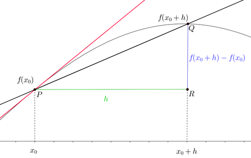 Figure 1. Geometric Interpretation
The thin curve is our \(f(x)\). As you can see, given a value \(x_0\) we find the point \(P=(x_0, f(x_0))\). If we consider an infinitesimal increase of \(h\), we get a second point: \(Q=(x_0 + h, f(x_0 + h))\). Now I’m fairly certain (I checked this morning) that it’s still true that
Through two points there passes exactly one line (at least in Euclidean geometry).
This line is called the secant and it’s the black line. Let’s go deeper and look at the explicit equation of the line:
where \(m\) is the slope of the line. Assuming we know two points on the line, we can write (if you want the proof, take a look here):
But wait, we do have those points:
and
So we write:
Sound familiar?!
So what we’re saying is that the difference quotient is nothing but the slope of the secant line.
As \(h\) becomes infinitesimally small, the distance between \(f(x_0+h)\) and \(f(x_0)\) shrinks.
This means that \(Q\) moves closer and closer to \(P\) until they become the same point.
Therefore, as \(h\) tends to \(0\), just like in the definition of derivative, the secant becomes the tangent, the red line in the plot.
All of this leads us to say that the limit of the difference quotient, or
the derivative among friends, represents the slope of the tangent line to the graph of the function.
- If the line slopes upward from left to right, then \(f'(x) > 0\) and the function is increasing.
- If it slopes downward from left to right, then \(f'(x) < 0\) and the function is decreasing.
- If it’s horizontal, then \(f'(x) = 0\) and the function is steady.
The slope of the line also tells us the rate of change. The steeper the line, the faster the function changes. For example, consider the function:
Its derivative is:
Given \(x=1\), we have:
and
Which means that at the point:
the function increases with a rate of \(2\), i.e., for every unit increase in \(x\), the value of \(f(x)\) increases by 2.
Here’s a graphical representation of what we’ve discussed:
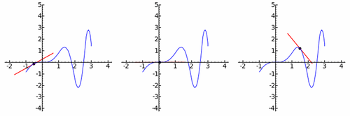 Figure 2. Graphical Behavior of the Derivative
From left to right, you can see the three cases: increasing function, constant function, and decreasing function.
Although there’s much more to say about derivatives, like their rules, I’ll just add that from this point on, I won’t use only the \(f'(x)\) notation for derivatives, but also the \(\frac{d f}{d x}\) notation, called the Leibniz notation. Why?! Because I’m a supporter of Leibniz’s claim to the invention of calculus... but that’s another story. Just know they’re two ways to represent the same thing.
So, we’ve covered the mathematical and geometric interpretation of the derivative. We’re missing the physical interpretation, but honestly, I’m not in the mood. So here’s the example below, figure it out from there.
From Definition to Action
Let’s consider a very simple example to better explain the concept of the derivative and its physical meaning. Suppose we’re driving a car, and our position over time is given by this function:
Then we have:
So:
Thus:
Finally, we consider the limit as \(h \rightarrow 0\):
We’ve now computed the derivative of the position function. But what does it represent?
Remember, the derivative measures the rate of change of the function.
In our case, it represents the rate at which position changes with respect to time.
We’ve thus obtained the velocity function.
Let’s analyze it in detail by looking at its value at different time instants:
- Suppose \(t=0\):
\(\frac{d s}{d t} = 10\) - Suppose \(t=5\):
\(\frac{d s}{d t} = -10 + 10 = 0\) - Suppose \(t=7\):
\(\frac{d s}{d t} = -14 + 10 = -4\)
At the initial moment (case 1), the velocity is \(10 \frac{m}{s}\), but after \(5\) seconds (case 2), we are instantaneously at rest. This means velocity is decreasing: we are decelerating. After \(5\) seconds (case 3), velocity becomes negative: we are moving backward, literally. So the car’s behavior is this: it was moving forward but slowing down, we came to a stop, and then began to reverse.
Who would have thought a simple formula could tell such a story? And guess what? We’ve only just scratched the surface.
The Dark Side of Change: Integration
The derivative is the infinitesimal change. We've said it again and again, and I hope the message has sunk in.
Now let’s pause for a moment to reflect: if the derivative measures the infinitesimal change of a function,
then by summing an infinite number of these tiny changes, we can reconstruct the original function.
Makes sense, right?
Excellent, what we’ve just introduced is the concept of the integral.
But beware, because here’s where things get tricky.
In fact, while with derivatives we have a nice formula to help us, here we don’t.
Integrals are more of a pattern matching game, the solution isn’t direct but stems from the question:
What is the function whose derivative gives the one I’m looking at?
That is, to solve an integral, we have to recognize it as the derivative of something.
But let’s start from the beginning.
In derivatives, \(h\) represented an infinitesimal increment. Now we change notation and use \(dx\) instead of \(h\).
We have the infinitesimal change, so we can estimate the variation:
From the derivative formula, we have:
and thus:
Graphically, what we’re calculating is the area of an infinitesimal rectangle under the function \(f'(x)\), where the height is given by the value of \(f'(x)\) at a given point, and the base is the infinitesimal increment \(dx\). You might be wondering why I used the approximation symbol instead of equality. Take a look at the image below.
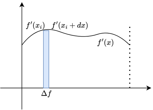 Figure 3. Infinitesimal Area
As you can see, a rectangle can never perfectly fit a curve, but the “narrower” the rectangle, that is, the smaller the \(dx\), the better the approximation. And for \(dx \rightarrow 0\), the approximation becomes equality.
As mentioned earlier, to recover the original function, we must sum all these areas. And how many are there? Since the increment is infinitesimal, it makes sense to think we have infinitely many increments. So we can write:
This sum is an approximation, and when taken to infinity, it becomes the integral. Mathematically, it’s written as:
This formula is the fundamental theorem of calculus and tells us, in simple terms, that the integral is the inverse operation of the derivative. The generic \(F(x)\) is called the antiderivative, and it's the function whose derivative gives back the argument (what we’re integrating) of the integral.
Now you might be asking: what the heck is this C?
If you apply the difference quotient to a constant function, you get \(0\).
This means that in differentiation, we lose all information about constants.
That’s why when we integrate, we always add the constant \(C\), to compensate for this loss of information.
What we just defined is called the indefinite integral. And yes, if there’s an indefinite one, there’s also a definite one. The definite integral doesn’t compute a function, but a number, and it’s written like this:
That is, the difference between the antiderivative evaluated at \(b\) and at \(a\).
What you just had the "pleasure" of reading is Riemann integration.
There are many others, like Lebesgue integration, but don’t worry, we won’t go into that. I’m tired, and I bet you are too.
Now we have everything we need for two examples.
Indefinite Integral
Suppose we have:
and we want to recover \(f(x)\), we get:
How do we get there?
The mental process should be: what is the function whose derivative is \(x\)?
Let’s apply the difference quotient to the resulting \(f(x)\) and see if it works!
To wrap up this example, the original \(f(x)\) could simply have been \(\frac{(x+h)^2}{2}\), or \(\frac{(x+h)^2}{2} + 1\), or even \(\frac{(x+h)^2}{2} + 100000\). Constant values are always lost in derivative calculations. So, when using an integral to move from a derivative to the antiderivative, we must account for those constants with a generic \(C\). Otherwise, you’ll lose a point on a five-point exam. Trust me...
Definite Integral
For this second example, besides applying the integral formula, I also want to show you why the idea of infinite summation of rectangle areas works.
Let’s suppose we want to compute the area under the function \(f(x) = 2x\) in \([0, 2]\).
Note that there’s no derivative symbol here. That’s because derivatives are the classic shadow consultant:
they’re there, doing all the work, but you don’t see or hear them (don’t worry, they don’t want to see or hear you either).
Back to the topic. Using the integral in its strict form, and aided by the table of indefinite integrals, we write:
So, the area under \(f(x) = 2x\) from \([0, 2]\) is \(4\), and the problem would be solved. But since I’m cruel, let’s apply the theory strictly and do that cursed infinite summation. We’re in the interval \([0, 2]\), and we want to divide it into infinitesimally small pieces \(dx\). We use:
where \(n \rightarrow \infty\), meaning we have infinitely many small pieces (or rectangles) of the interval. The area of one piece is:
and summing all these areas gives:
Now pay attention here. We must evaluate each point on the graph of \(2x_i\). But this graph is split into many \(dx\) as described. The first rectangle spans \([0, dx]\), the second \([dx, 2dx]\), and so on. We said \(dx = \frac{2}{n}\), right? So the first rectangle is \([0, \frac{2}{n}]\), the second \([\frac{2}{n}, 2 \cdot \frac{2}{n}]\), and so on. Noticing the pattern? Please say yes... To summarize, the base points of the rectangles follow the rule:
To better visualize this, refer to the image below:
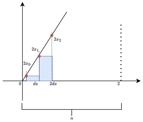 Figure 4. Domain Partitioning
Now we can compute \(f(x_i)\) at each point:
- At \(i=0\)
\(2x_i = 2 \cdot 0 \cdot \frac{2}{n} = 0\) - At \(i=1\)
\(2x_i = 2 \cdot 1 \cdot \frac{2}{n} = \frac{4}{n}\) - At \(i=2\)
\(2x_i = 2 \cdot 2 \cdot \frac{2}{n} = \frac{8}{n}\) - ...
So in our summation, we can substitute
with its value:
yielding:
Only \(i\) is tied to the summation. To solve, we sum infinite \(i\) values:
How much is this sum? If you studied calculus and don’t know, you should be ashamed. For everyone else: it has a well-proven solution by good ol’ Gauss:
So we have:
and since \(n \rightarrow \infty\), we write:
We got exactly the same result.
Didn’t I tell you that an integral is the sum of infinite rectangle areas!?
What’s that? You still want a (completely uncalled-for) physical interpretation? Fine, remember when we said that velocity is
the derivative of position with respect to time? Well, since integration is the inverse of derivation, integrating velocity (yes, we have velocity function) over time
gives us position. So, if we traveled at a speed of \(2t\) for \(2\) seconds, how much distance would we cover? Exactly
\(4\) meters.
When Change Becomes Law
Alright, now things are getting serious, but let’s stay calm.
In the previous section, we looked at the derivative as the main tool to measure how a function changes over time. We also saw that, knowing a derivative, we can (at least theoretically) recover the original function using the integral.
But what happens if, instead of a “nice” derivative ready to integrate, we’re given a rule that tells us how that derivative behaves,
perhaps depending on the same variable? In other words: what if we only know an equation that links the rate of change
to the function itself, without knowing either explicitly? Welcome to the world of ordinary differential equations, or as friends call them: ODEs.
ODEs don’t tell us what the function looks like, but how it evolves over time.
They’re not the ID photo of a phenomenon, but its dynamic behavior.
And be warned: don’t be fooled by the word “equation.” In an algebraic equation we look for a number, in an ODE,
the solution is an entire function. It’s worth noting that when we speak of differential equations, we’re talking about a vast world in which ODEs are just a small part.
There are PDEs (partial differential equations), SDEs (stochastic differential equations), and so on.
And each one, in its own way, will hurt you. Hurt you deeply. But since I’m still too young to die from this,
let’s focus on ODEs for now, we’ll see what comes next. But what does an ODE look like? An ODE is like COVID... you can’t see it or hear it, but it’s out there threatening you, and someone will deny its existence.
Basically, it’s an equation that involves at least one derivative and tells us how something should change.
Everything revolves around a single independent variable, usually time \(t\) (but it could also be space, temperature, or how much will to live you’ve got left).
Instead of knowing the function \(y(t)\) directly, we know its derivative, in other words, how \(y(t)\) changes over time.
Let’s start with the simplest ODE example:
Where:
- \(t\) is the independent variable (often time),
- \(y\) is the unknown function we want to find,
- \(f(y(t), t)\) is the function describing how \(y(t)\) changes over time.
For example:
As you can see, we don’t know the function \(y(t)\), but we know that \(y\) grows proportionally to its own value with a factor of \(3\). The goal, then, is to find the function \(y(t)\) that satisfies this growth law. In this case, the solution is:
How did I find that? We’ll figure it out soon...
For now, let’s highlight a few more facts about ODEs.
The one we just saw is an ordinary differential equation of first order, linear, explicit, and with constant coefficients.
- First order means it contains only the first derivative \(\frac{dy}{dt}\), not higher ones like \(\frac{d^2y}{dt^2}\).
- Linear means that \(y\) and its derivatives appear to the first power, there are no powers, products, or non-linear functions of \(y\).
- Explicit means the derivative is isolated on one side of the equation, like: \(\frac{dy}{dt} = f(t, y)\).
- Constant coefficients means the terms multiplying \(y\) or its derivatives are fixed numbers and not functions of \(t\).
Now that you’ve seen what a nice and cuddly ODE looks like, let’s balance things out with one that’ll make you curse:
Here we have the complete opposite:
- It’s second order, meaning \(y(t)\) has been differentiated twice, as seen in the term \(\frac{d^2y}{dt^2}\).
- It’s non-linear since \(y\) is squared.
- It’s implicit because the derivative is multiplied by a factor of \(t\).
- It has variable coefficients because \(y\) or its derivatives are multiplied by a value that changes (in this case, \(t\)).
Not Great, Not Terrible. Just... Cauchy.
Earlier I said that the solution to an ODE is a function, and that’s true. But I never said it’s not possible to know the value of \(y(t)\) at a specific time \(t\). All we need is a starting point, that is, we need to know the value of \(y(t)\) at least at one moment in time. Once we have that, we can know its value everywhere. This starting point is called an initial condition, and if we have it, we’re dealing with a Cauchy problem or IVP (Initial Value Problem). An IVP is structured like this:
That is, after solving the ODE, we know that at time \(t = k\), \(y(t)\) is \(z\).
From Law to System
Unfortunately (or fortunately), the world doesn’t work with just one variable. When we want to describe multiple interacting phenomena, we need to move from a single equation to a system of ODEs. A system of ODEs is a set of equations that describes multiple evolving quantities, all interconnected. For example:
Here, the functions \(x(t)\) and \(y(t)\) influence one another. You can’t just solve one and then the other: they’re coupled and must be solved together. And if we also have initial conditions for both ODEs, then we’re dealing with an IVP:
ODE Hall of Fame
Yes, I know, up to this point it’s all been complicated and abstract, but even if it doesn’t seem like it, we’re surrounded by ODEs. ODEs everywhere. An example? Newton’s famous formula, the second law of motion (yeah yeah, we’ll give Leibniz a break):
Even though it doesn’t look like it, acceleration is the derivative of velocity, which in turn is the derivative of position over time. So acceleration is the second derivative of position over time, and we can write:
Another famous example is the Lotka-Volterra system, or the predator-prey model. This system of ODEs represents the equilibrium created in an environment with prey and predators (e.g., rabbits and foxes). The system looks like this:
The graphical behavior of this system is shown in the diagram below, called a direction and phase diagram:
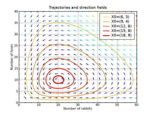 Figure 5. Lotka-Volterra Direction and Phase
Note: the two graphs can be shown separately, but for brevity, you get them together here. The direction field is used for first-order ODEs and visually represents how solutions behave at every point in the plane, assigning an arrow tangent to the curve at that point. So now you know it shows not just the direction but also the rate of change of the ODE. If that’s still unclear, don’t tell me, otherwise all of this was pointless.
The phase diagram, on the other hand, is used for ODE systems and shows the evolution of relationships between variables. Back to the graph: \(x\) and \(y\) are foxes and rabbits. As you can see, their interaction forms a closed system. When foxes increase, there are too many predators, and rabbits decrease. Once rabbits become too few, there’s not enough food for the predators, so they decrease too, giving rabbits a chance to repopulate. The different colored lines represent the same system (i.e., the same behavior), but under different initial conditions.
Let’s move on to the last famous ODE of the day. Ever heard of the butterfly effect? That idea that small actions can lead to large and unpredictable long-term consequences? Well, that effect originates from the following ODE system called the Lorenz system:
Here’s what its graph looks like:
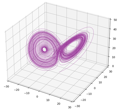 Figure 6. Lorenz Attractor Phase
From the shape, you can guess why it’s called the butterfly effect. But what’s fascinating about this ODE system is this: the graph never passes through the same trajectory twice. Also, since the variables influence each other through multiplicative factors, a tiny variation grows significantly over time \(t\), which is why it’s associated with chaos. A final point worth noting is the presence of attractors, points that pull solutions of the ODE toward them. Even though, like lightning, the Lorenz system never strikes the same point twice, the system is attracted to those points, orbiting around them. A system with the opposite behavior is called a repulsor, and you can see one below:
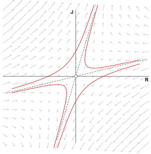 Figure 7. Repulsor
But now I’ll end this paragraph, there’s a storm coming.
To Wrap Up
I know this article was mathematically a bit heavy, and that there was nothing about computer science, neural networks, or metaheuristics. But hey, if I put it under the Theory and Mathematics section, there must be a reason, right? Like it or not, this is the math that’s hiding behind it all, this is it. And if you’re the type that says:
ooooh I love working with AI, it’s sooo cool, love it...
but you hate math and your deepest understanding is import sklearn,
you’ve definitely chosen the wrong career.
Jokes aside, don’t rest on your laurels thinking:
I made it to the end
because it’s not over yet. There’s much more to discuss, like for instance:
How the heck do you solve ODEs?
But since this is just one in a series of articles, we’ll save that answer for later, let’s just swallow this bitter pill for now. In the meantime, you can head over to this repo to see some of the topics covered in action.
Until next time.