

Here we are again with the second part of the series dedicated to Neural ODEs. If the first article was a mental beating this one will be a bit less so. But don’t get your hopes up: it’s still no walk in the park. We’ve already sunk our hands into the mire of derivative, integral, and differential equation. And now, since we’ve already ruined our manicure, we might as well go all the way and answer one of the unresolved questions from the first article. So without further ado (or bloodhound), let’s begin and see how to solve an ODE.
ODE To The Method
I know, I can feel it, you couldn’t wait to find out how to solve an ODE and finally, here we are. How do you solve an ODE? The short answer is: it depends. As always in life, there are two options: one elegant and one brutal.
On one side we have the analytical methods. They’re classy and well-dressed, like an intern at a Big 4 firm. They’re the methods that give you an exact formula for the solution. Now a question arises. If they’re so good and perfect, why do we need alternatives? Because, just like an intern at a Big 4, when the going gets tough these methods aren’t enough and you need to ask for help from others.
And here come the numerical methods. The bold ones in the room. Let’s just say it, they’re like junior trainees at a Big 4 (Big 4 friends, of course this is just a joke, peace and love.). They don’t care about elegance or exact formulas, head down and they get the job done. They move forward step by step, estimating the solution point by point. They’re not exact, that’s true. But sometimes, they’re the only viable way.
In short, choosing the right method depends on two things:
- On you: maybe you don’t feel like sweating over an analytical solution or simply don’t need it.
- On the problem: because some ODEs simply don’t have an analytical solution. And when that happens, what you want is worth about as much as a two of clubs when spades are trump.
Analytical Methods
Let’s start with the pretty boys of the bunch. Analytical methods are able, at least when everything goes smoothly, to extract the closed-form expression of the function that solves the equation. These methods are only applicable under specific, often ideal, conditions that you’ll typically find only in university textbooks. There’s no single method available instead, depending on the structure of the ODE, we have several at our disposal:
- Separation of Variables method
- Integrating Factor method
- Similarity method
- Laplace Transform method
- ...and many more, but trust me, the list is long
Will we look at all of them? Absolutely not. We’ll go over just the first two to show I’m not making this stuff up. But if you want a complete and detailed overview, I recommend reading this.
Separation of Variables
The separation of variables method is one of those techniques that make you go “okay, that’s cool, but when would I ever use it?”. In fact, it’s applicable only when an ODE can be written like this:
Having this structure allows us to do the following:
That is, we multiply both sides of the equation by \(dt\) and divide both by \(f(y)\). Basically, we’ve separated the equation, putting all \(y\)-related terms on one side and all \(t\)-related terms on the other. To get a better feel for this, try playing with the following ODE:
Swear, curse, and bang your head against the wall, you’ll never be able to separate \(y\) from \(t\). In at least one side of the equation, there will always be an intruder, whether it’s related to \(y\) or to \(t\).
At this point, all that’s left is to integrate both sides of the equation, solving the ODE:
Example
Great, we can finally look at an example. In this paragraph I casually dropped an ODE along with its solution, without telling you where it came from. Let’s pick it up again:
This fits very well with separation of variables, it’s already written in the form we need:
where:
- \(f(y) = y(t)\)
- \(g(t) = 3\)
So we do our little magic trick to separate the \(y\) terms from the \(t\) terms:
Now that we’re wizards with derivatives, when we see \(d-something\), we know it’s an infinitesimal, and we need to integrate to find the antiderivative. So we integrate both sides, indefinitely:
Using the table of notable integrals, we can easily solve these:
from which:
Since \(C_2\) and \(C_1\) are arbitrary constants, which can take any value (reflect on this point here) we can, with a light heart, set:
So the solution becomes:
To isolate \(y\), we need to invert the natural logarithm, so we raise both sides as powers of \(e\) and get:
Following the same principle as before, \(e^C\) is an arbitrary constant, so we can simply rename it:
and therefore
This proves that I wasn’t talking nonsense in part 1. Everything checks out, and the world can resume spinning. Now we’re left with the bitter taste of “okay, but what’s the value of K?” The problem doesn’t provide enough information, so as posed we can’t know it. To determine \(K\) we’d need a Cauchy problem. What’s left...? Ah yes, to show the graphical behavior. Here it is
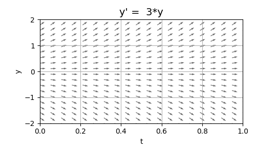 Figure 1. Plot of \(y=K \cdot e^{3t}\)
Let’s comment on this graph. As you know, or at least should from part one, it’s a direction field graph. Even though we know the general form of the solution, without knowing the value of \(K\) we can’t trace the exact curve. However, the direction field helps us: it shows how solutions behave for different values of \(K\), even without knowing them explicitly. What we notice is that there are three families of solutions:
- The increasing family: arrows for \(y>0\) diverge upwards.
- The decreasing family: arrows for \(y<0\) diverge downwards.
- The constant family: consisting of a single lonely member, always zero, corresponding to \(y=0\).
Integrating Factor
Remember that little ODElette (who’s not the wife of ODEman... ok, I disgust myself), which in the previous paragraph couldn’t be solved? I mean this one:
Quick note: \(y\) is always a function of time, so you might read \(y\) instead of \(y(t)\), but they’re entirely equivalent.
Well, with the integrating factor method we can go where separation of variables couldn’t. This method requires the ODE to be first-order linear (read more here), and it must be written in the form:
Formula 1. Base Form for Integrating Factor
At this point, the method requires us to define the integrating factor as:
and we multiply every term of the ODE by \(\mu (t)\):
Formula 2. Integrating Factor
Now we use a math trick. Let’s take the product rule for derivatives:
Formula 3: Product Rule
Since we’re dealing with a first-order ODE, we have:
so that:
since we’re differentiating an integral, and
because \(e\) is the base of the natural logarithm. Therefore:
Plugging this into Formula 3, we get:
Since last time I checked, Formula 2 still holds, we can write:
Integrating both sides gives:
Finally, ladies and gentlemen, dividing by \(\mu(t)\) we get the final formulation of \(y\):
Formula 4. Integrating Factor Solution
As we’ve seen, with not a few hurdles let’s be honest, when we can apply the integrating factor, we have a nice little “formula” ready to explicitly solve the elusive \(y\). I’d say it’s time to look at an example.
Example
The ODE we wanted to solve was this:
Right!? Great, even better! This one lends itself to the integrating factor method. So let’s revisit the ODE, but this time we solve a Cauchy problem, and assume we not only have the ODE, but also the value of the solution \(y(t)\) at \(t=0\), which we’ll assume to be \(0\) (but it could also have been \(y(t)=5\) at \(t=214\), we just need to know at least one value of the function at a specific time):
Let’s start from the ODE:
So:
- \(p(t) = -2t\)
- \(q(t) = t\)
From the integrating factor solution formula, we need to compute:
Which gives:
Now we need to solve:
I can feel it, the terror gripping the hearts of anyone who took Calculus 1, because solving this integral requires the substitution method, which I won’t explain here but I’ll leave you with a source to dig deeper. So let’s set:
Back to original variables:
and so:
Returning to our \(y\):
Where, being arbitrary constants, we set:
Thus:
Remember we’re solving a Cauchy problem where at \(t=0\), \(y=0\), so:
Thanks to the initial condition, we’ve found the value of \(K\), which lets us compute \(y\) at any point in time. If you were paying attention, you know the value of \(y\) at \(t=0\). So let’s now compute it for \(t=1\):
Exactly as I hinted, having an initial condition allows us to determine the value of the ODE at any moment in time \(t\). Of course, the initial condition can alter the ODE’s behavior. Let’s take a look at the direction field and phase diagram.
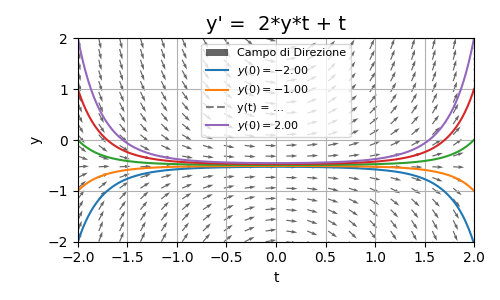 Figure 2. Plot of \(y=-\frac{1}{2} + K \cdot e^{t^2}\)
Remember when I said in part one that phase diagrams are used for systems of ODEs? Well, that’s not entirely true, because even a single ODE, if it comes with an initial condition, produces a well-defined curve in the \((y,t)\) plane. That’s exactly what I’m doing here. But why is it possible in this case? Simply because now we have a Cauchy problem, not just a plain ODE. So with an initial condition, I can compute \(K\) and see the behavior of \(y\) over time with \(K\) known. Thus, the direction field shows us all possible solutions: the initial value determines which of these, our
will follow. In our case, the initial condition is \(y(0) = 0\) which implies \(K=\frac{1}{2}\). In the plot, this specific case is shown by the green line (and no, don’t switch to RAI 1). Here too, just like before, we have three distinct families:
- \(y > -\frac{1}{2}\): Field lines decrease rapidly (see the steepness of the arrows) and then start to increase again.
- \(y < -\frac{1}{2}\): Field lines increase rapidly and then start to decrease again.
- \(y = -\frac{1}{2}\): The function remains constant and zero-valued
If you want to verify for yourself, try setting the initial condition \(y(0) = -\frac{1}{2}\) and go through the math. You’ll find that it implies \(K=0\).
To Wrap Up
I swear I started with the best intentions, but I got a bit carried away. So here we are, at the end of a second part that was mathematically pretty intense.
As for the third part, well I can’t promise it’ll be any easier, but you’ve started dancing, so now KEEP DANCING!
As always, here’s the link to the repo.
Oh, and in case it wasn’t obvious, the next article in our beloved series will be about numerical methods.
Until next time.