

There comes a time in the life of every mathematician, engineer, and mythological figure alike when
You like analytics, huh!? Then take this ODE.
And it smacks you with a nonlinear, coupled, implicit one, with coefficients changing like the Hogwarts staircases. The only thing you can do is not solve it. Not even by praying to the good souls of Gauss, Leibniz, and whatever other mathematicians you worship. Or at least, that was true until the advent of numerical methods. Not very elegant, often messy, but incredibly effective. They won’t give you any closed-form formulas to brag about, but if you settle for an approximate result, you really can’t complain. After all, although it might not seem like it, we are surrounded by approximations: when you use Google Maps (that tells you’ll arrive in 10 minutes and you get there in 17), when you add a pinch of salt (where “pinch” means a tablespoon), when you read my blog (which is supposed to be educational but helps me more to remember than you to learn)...
But enough chit-chat, since you’re probably on the edge of your seat, let’s finally look at these famous numerical methods. But first, if you haven’t already, go check out Part 1 and Part 2.
ODE in Small Steps
Let's revisit the much-praised Lotka-Volterra system introduced here.
where:
- \(x(t)\) is the number of prey (e.g., rabbits).
- \(y(t)\) is the number of predators (e.g., foxes).
- \(\alpha\) is the prey growth rate. It describes how quickly prey reproduce in the absence of predators (which, in the case of rabbits, is apparently quite high according to legend).
- \(\beta\) is the predation rate. It indicates how often prey are killed by predators.
- \(\delta\) is the conversion rate. It tells how many new predators are born per prey eaten and digested.
- \(\gamma\) is the predator mortality rate. It represents the natural death rate of predators in the absence of prey. If they don’t eat, they starve.
There is no known analytical method to symbolically solve this system, so we turn to numerical methods. These are strategies to obtain an approximate solution, using small, discrete, and hopeful steps. All thanks to the great Euler, who, in addition to giving us the iconic tattoo
(no seriously folks, stop getting it tattooed if you don’t even know what pi is), also gave us the progenitor of all numerical methods: the Euler method. The convergence of this method was proven by the venerable Cauchy and later generalized by the eminent Runge and Kutta with the family of RK methods. Basically, everyone here is great, and the world of numerical methods is more crowded than TikTok’s algorithm. There are many more we could cover, but we’ll stick to a select few.
Euler's Method
Let’s go back to the Taylor series expansion. Remember? I already talked about it here. The Taylor series is like a wildcard, it shows up everywhere.
Let’s consider in particular a first-order expansion, i.e.,
where
In other words, we are evaluating the function at \(x\), using derivatives calculated at a point \(a\) that is offset from \(x\). Now let’s consider a generic Cauchy problem:
and recall the definition of derivative. For \(h \rightarrow 0\) we can write:
Does it look familiar? Exactly, a first-order Taylor expansion, where:
- \(x = t + h\)
- \(a = t\)
So we calculate the derivative at time \(t\) and use it to estimate the function at \(t+h\). Now let’s go further and assume we start at time \(t_0\), which we know because we’re solving a Cauchy problem. We take a tiny step \(h\) forward and land at \(t_1\). Thus:
where
Once we have \(t_1\), we can move to \(t_2\) in the same way:
where
Get the idea? We can generalize it like this:
Formula 1. First-Order ODE Expansion
Thus:
Formula 2. Time Discretization
Where:
- \(t_0\) is the initial time
- \(t_{n+1}\) is the final time
- \(h\) is the integration step size, freely chosen
- \(n\) is the number of iterations
In short, we’re discretizing time. The smaller \(h\) is, the more accurate the method, but also more computationally expensive.
Going back to the Cauchy problem:
we can plug this into Euler’s method and get the final formulation:
Formula 3. Explicit Euler Method
That’s the formula for the Explicit Euler Method. Why “explicit”? Because we use only known values. Suppose we want to compute \(y(t_1)\):
- \(y(t_0)\) is given by the Cauchy problem
- \(f(y(t_0), t_0)\) can be calculated by simple substitution
And of course, if there’s an explicit method, there’s also an implicit one, whose formula (without proof) is:
Formula 4. Implicit Euler Method
It’s called implicit because, as you can see, the value we want to compute, \(y(t_{n+1})\), appears on both sides of the equation. It’s not always easy to solve. In some cases, iterative methods like the successive substitution method are needed. But that’s beyond the scope of this article, and since we’ve already made life complicated enough, I’ll leave it to your curiosity to dig deeper.
Euler Example
All of this has been a bit too theoretical so far, I know, so let’s look at something practical with an exercise. Let’s consider the following Cauchy problem representing exponential decay. It may seem pointless, but many natural phenomena follow this law, such as radioactive decay, capacitor discharge in RC circuits, etc.
where \(k\) is the decay rate, and in this case, we choose it ourselves. The solution to this ODE is:
If you want the steps, do them yourself. You already know the tools to solve it. I chose this ODE (which can be solved analytically, as you've seen) to show the difference between an exact and a numerical solution. Let’s see the values at \(t=1\) and \(t=2\).
Now let’s solve it using Euler’s method. From the time discretization formula, we already know how many steps we need using \(h=0.1\), initial time \(t_0=0\), and final time \(t_n=2\):
For clarity, let’s go step by step. The value at \(t_0\) is given in the Cauchy problem, so:
- Step \(n=1\)
$$ t_1 = t_0 + 1 \cdot 0.1 = 0.1 $$
- Step \(n=2\)
And so on. Trust me when I say the results are those shown in this table:
Now let’s see what happens with \(h=0.5\). I won’t go step by step because you know how it’s done now, so just take this table:
Here’s a summary comparison between the analytical solution and the two numerical approximations:
- \(y(t)\) is the analytical solution
- \(E(h=0.1)\) is Euler with \(h=0.1\)
- \(E(h=0.5)\) is Euler with \(h=0.5\)
As you can see, apart from \(n=0\), the known solution, \(h=0.1\) gives a much better approximation than \(h=0.5\), but it also requires 20 steps compared to just 4 in the latter case.
All of this can be summarized by the following image:
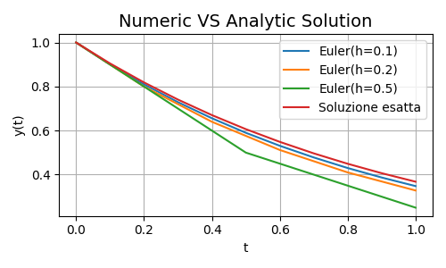 Figure 1. Results Comparison
The exact solution is the red one, and as \(h\) decreases, the approximation gets better and better. Alright, time to move on to the next round where the Runge-Kutta methods will knock you out.
The Mans... RK Family
Let’s give credit where credit is due: Euler’s method is the patriarch of all numerical methods. But is it really that good? Well, as always... it depends. For instance, on the type of problem you’re dealing with. For problems that are too complex, it can fail miserably. So yes, it’s good and dear, but let’s be honest, it’s getting old. We need fresh blood, brave and strong youngsters. That brings us to the Runge-Kutta methods, or simply RK.
RK methods are like a sprawling dynasty, and each has its own quirks. The only certainty, besides death, is that they keep Euler’s core idea: proceed in small steps.
Let’s go back to the Taylor expansion. As you’ll remember, the higher the order of expansion, the better the approximation. RK methods are built exactly on higher-order Taylor expansions. So Euler can be viewed as a method of order 1, i.e., RK1, or first-order Runge-Kutta. Now let’s see what happens when we go beyond first order and move to the second, starting from the First-Order Formula:
Given that
Formula 5. Second-Order ODE Expansion
We can then use the definition of the first derivative and expand \(f'\) using a finite difference:
But from Euler’s method we know that
Substituting in:
Substituting again into the Second-Order Expansion, we get:
So let’s define:
and we obtain the so-called RK2 Method, or Heun’s Method:
Formula 6. Heun’s Method
Following the same logic, you can derive higher-order methods by expanding Taylor’s series further:
- RK3 or Shu-Osher
- RK4
- RK5 or Dormand-Prince
- ... and many more.
Given its importance, we must include the RK4 formulation, it’s an excellent balance between precision and computational complexity:
Formula 7. RK4 Method
Note that, just because I care, we’ve only considered explicit methods here. But sticking our heads in the sand doesn’t mean that implicit RK methods (yes, they exist) can’t hurt you.
RK Example
If you’ve made it this far, you’ve probably heard about Lotka-Volterra a bazillion times. And now that we can, why not solve it?! So let’s take the following setup:
Obviously, after all the rambling above, we’ll use numerical methods with:
Specifically, we’ll apply both Heun and RK4. Don’t worry, this is just to show you how they work, so we’ll only carry out one step.
- Heun, \(n=1\)
Remember, Lotka-Volterra is a system of two ODEs, so it gets a little more involved, but nothing crazy. Don’t panic. Let's start by calculating \(k_1\) and \(k_2\). Since we have two ODEs, we’ll compute:
- \(k_1^x, k_2^x\) for the first ODE
- \(k_1^y, k_2^y\) for the second ODE
Substituting:
The sharpest among you may wonder why \(t+h\), required for computing \(k_2\), doesn’t appear anywhere. Simple: all the ODEs in the system don’t explicitly depend on time \(t\), so it’s irrelevant for the computation. But if it did matter, the current time would be calculated using the Time Discretization Formula shown in the previous section.
- RK4, \(n=1\)
Using the same idea, we calculate:
- \(k_1^x, k_2^x, k_3^x, k_4^x\) for the first ODE
- \(k_1^y, k_2^y, k_3^y, k_4^y\) for the second ODE
Substituting:
Yeah, I know, it's a lot and seems overly complicated, but once you have the method’s formula, it’s just about making the right substitutions carefully.
Just like with Euler’s method, let’s provide a comparison table here. This time, we’ll group by method rather than \(h\), and compare the results of RK4, Heun, and Euler. As we cannot compute the analytical solution here, all we have are approximations.
As seen from the table, Heun and RK4 give very similar results, with differences appearing only after \(t=2\) seconds. In contrast, Euler starts to deviate poorly as early as \(t=0.1\). The following image shows the phase behavior:
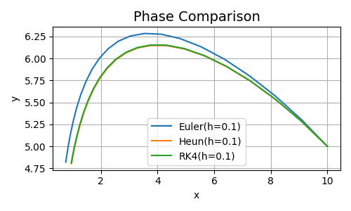 Figure 2. Results Comparison at \(t=2\)
Finally, let’s see what happens when we extend the time from \(t=2\) to \(t=15\).
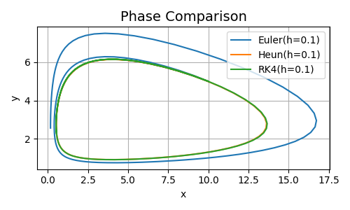 Figure 3. Results Comparison at \(t=15\)
As you can see, Heun and RK4 have very similar, theoretically consistent behavior, forming a closed orbit (read previous posts if you don’t remember what that means). Meanwhile, Euler accumulates error so heavily that its solution goes completely off track.
To be thorough, here’s the time series of prey and predator populations, i.e., \(x\) and \(y\), over time \(t\):
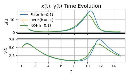 Figure 4. Behavior of \(x\) and \(y\) over time \(t=15\)
To Wrap Up
Here we are at the end of this third article. By now, you should know (or at least remember, if you already had the knowledge) what derivatives, integrals, differential equations, and numerical methods are. There’s so much more to say, but I tried to keep it concise. No need to thank me. In any case, we now have all the ingredients to talk about Neural ODEs. And in case you were wondering, yes, there will be plenty of math there too. As always, I’ll end with the link to the repo where you can see the code behind everything we’ve discussed.
Until next time.