

Here we are. We've reached the fifth and final part of the NODE series. Though take that statement with a grain of salt, if I run out of space, you might get a sixth one too. In any case, in this (hopefully) final part, we'll look at some code and an actual application of a NODE. Before we begin, if you've landed on this page without reading the previous ones, I strongly recommend going back and checking them out. You can find the links to the earlier articles here. With that said, let's dive in.
From NODE to Code
If there's one thing we've learned (or at least should have), it's that NODEs differ from standard neural networks not so much in terms of architecture, but in the way these architectures are used. With that in mind, let's not be discriminatory. Don't treat NODEs any differently, they can do everything a classical neural network can do. They can be used for classification problems, regression, and even generation. That said, due to their continuous nature, they are naturally better suited for certain use cases, though there's nothing stopping you from using them whenever, however, and for whatever you want. I’m certainly not going to stop you. In the examples I’ll show, I’ll use them in their natural habitat: forecasting, and I’ll compare the results with those produced by a classical neural network.
(Again) Lotka-Volterra
Let’s start with this first use case. Suppose we have a Time Series, whose nature is unknown to us. All we know is that we have a list of numbers thrown together. We know what those numbers represent, but shhh, the NODE has no idea what they mean. This list of numbers is our starting point, the data we’re going to use to train our NODE. And since, unfortunately, this data doesn't generate itself, we’ll have to create it manually. Wondering how? Nothing could be easier. We’ll take our good old Lotka-Volterra dynamic model and feed it to an ODESolver. If you don’t know how this model is defined, go check out part 3.
But enough talk, let’s look at some code and create a class LotkaVolterra that extends a generic
DatasetProvider, where we define the system’s dynamics and how to generate the data.
Dataset Creation
class LotkaVolterra(DatasetProvider):

    def __init__(self, n_train: int = 80, noise_std: float = 0.01,
                 t_train_range: tuple[float, float] = (0.0, 6.0),
                 t_extra_range: tuple[float, float] = (6.0, 10.0),
                 n_extra: int = 200, n_resamp: int = 200,
                 alpha: float = 1.5, beta: float = 1.0,
                 delta: float = 0.75, gamma: float = 1.0,
                 initial_values: tuple[float, float] = (2.0, 1.0)) -> None:
        super().__init__(initial_values=initial_values, n_train=n_train, noise_std=noise_std,
                         t_train_range=t_train_range, t_extra_range=t_extra_range, n_extra=n_extra,
                         n_resamp=n_resamp)
        self.alpha = float(alpha)
        self.beta  = float(beta)
        self.delta = float(delta)
        self.gamma = float(gamma)

    ...

    def dynamics(self, t: torch.Tensor, state: torch.Tensor) -> torch.Tensor:
        x1, x2 = state[0], state[1]
        x1dt = self.alpha * x1 - self.beta * x1 * x2
        x2dt = self.delta * x1 * x2 - self.gamma * x2
        return torch.stack([x1dt, x2dt]).to(self.dtype)

    def _solve_at(self, t_grid_np: np.ndarray, method: str, dynamics: Callable) -> np.ndarray:
        ...
        sol = odeint(dynamics, self.x0_t, t_tensor, method=method, rtol=self.r_tol, atol=self.a_tol)
        ...
        return sol

    def __call__(self, method: str, dynamics: Callable) -> DataObject:
        t_train = np.sort(rng.uniform(*self.t_train_range, size=self.n_train))
        x_train_true = self._solve_at(t_grid_np=t_train, method=method, dynamics=dynamics)
        x_train_noised = x_train_true + self.noise_std * rng.standard_normal(x_train_true.shape)

        t_test_extra = np.linspace(*self.t_extra_range, self.n_extra)
        x_test_extra_true = self._solve_at(t_grid_np=t_test_extra, method=method, dynamics=dynamics)

        t_test_resamp = np.sort(rng.uniform(*self.t_train_range, size=self.n_resamp))
        x_test_resamp_true = self._solve_at(t_grid_np=t_test_resamp, method=method, dynamics=dynamics)
        x_test_resamp_noised = x_test_resamp_true + self.noise_std * rng.standard_normal(x_test_resamp_true.shape)

        return self._create_dict(t_train, x_train_noised, x_train_true, t_test_extra, x_test_extra_true, t_test_resamp, x_test_resamp_true, x_test_resamp_noised)

    def prepare_data(self, data: DataObject, shuffle: bool = True, use_noise: bool = True, train_K_max: Optional[int] = None) -> Loaders:
        out = {}

        if train_K_max is None:
            ds_train = self._build_pairwise_transitions(data["t_train"], data["x_train_noised" if use_noise else "x_train_true"],
                                                        data["x_train_true"], device=device)
        else:
            ds_train = self._build_multi_horizon_transitions(data["t_train"], data["x_train_noised" if use_noise else "x_train_true"],
                                                             data["x_train_true"], K_max=train_K_max, device=device)
        out["train"] = {"dataset": DataLoader(ds_train, batch_size=batch_size, shuffle=shuffle)}

        ds_resamp = self._build_pairwise_transitions(data["t_test_resamp"], data["x_test_resamp_noised" if use_noise else "x_test_resamp_true"], data["x_test_resamp_true"], device=device)
        out["resamp"] = {"dataset": DataLoader(ds_resamp, batch_size=batch_size, shuffle=False)}

        ds_extra = self._build_pairwise_transitions(data["t_test_extra"], data["x_test_extra_true"], data["x_test_extra_true"], device=device)
        out["extra"] = {"dataset": DataLoader(ds_extra, batch_size=batch_size, shuffle=False)}

        return out
Yes, I know, it's a lot of code. But let me explain. In the constructor, in addition to passing the parameters needed to define the system, we also provide information about how we want our dataset to be built:
t_train_range: Represents the time range from which we want to draw the training and testing samples.n_train: Indicates the number of training samples we want to generate.n_resamp: Indicates the number of test samples we want to generate.noise_std: Used to dirty up the train and test data. Because what’s life without a bit of challenge?t_extra_range: Represents the time range for which we want to perform forecasting.n_extra: Indicates the number of samples we want to predict in the forecast range.
So if we consider the following lines:
DataCreator = LotkaVolterra
params = {
    "n_train": 350,
    "noise_std": 0.01,
    "t_train_range": (0.0, 12.0),
    "t_extra_range": (12.0, 18.0),
    "n_extra": 300,
    "n_resamp": 200,
}
data_creator = DataCreator(**params)
data = data_creator.prepare_data(data)
What we're asking for is a dataset composed of:
- \(350\) training samples randomly drawn from the time range \((0, 12)\) seconds, along with their corresponding timestamps.
- \(200\) test samples randomly drawn from the time range \((0, 12)\) seconds, along with their corresponding timestamps.
- \(300\) forecast samples in the range \((12, 18)\) seconds (used only to check if predictions are correct), along with their corresponding timestamps.
These datasets are structured like this:
idx   t_i      x_i                  t_next   x_next               dt
--------------------------------------------------------------------------------
0     0.023    [ 1.986 -0.044]      0.118    [ 1.986 -0.235]      0.095
1     0.118    [ 1.968 -0.245]      0.159    [ 1.975 -0.314]      0.041
2     0.159    [ 1.986 -0.314]      0.160    [ 1.975 -0.317]      0.001
3     0.160    [ 1.971 -0.318]      0.200    [ 1.96  -0.394]      0.040
4     0.200    [ 1.988 -0.383]      0.211    [ 1.956 -0.415]      0.011
5     0.211    [ 1.948 -0.398]      0.306    [ 1.908 -0.593]      0.094
...   ...      ...                  ...      ...                  ...
where:
- \(t_i\): The current timestamp.
- \(x_i\): The system state at the current timestamp, computed both with and without noise (for
trainandtest). - \(t_{next}\): The next timestamp.
- \(x_{next}\): The state at the next timestamp. In the case of
train, this is the state \(K\) steps ahead, where \(K\) is a random integer. - \(dt\): The delta between the two timestamps.
By plotting this data, we get the following image:
 Figure 1. True and Noisy Training Dataset
If you're wondering how we actually solve the dynamics, we use the odeint method from the torchdiffeq library,
which provides high-level methods for working with NODEs. This method implements various ODE solvers,
and in our case we used dopri5.
Network Definition
Since the main goal is to compare results under equal conditions, we used two almost identical networks. Let’s see why they are almost identical and not completely identical.
def lotka_volterra_nets():

    def create_net(is_node: bool):
        input_dim = LotkaVolterra.get_dim() if is_node else LotkaVolterra.get_dim() + 1
        return nn.Sequential(
                torch.nn.Linear(input_dim, 16),
                torch.nn.Tanh(),
                torch.nn.Linear(16, 32),
                torch.nn.Tanh(),
                torch.nn.Linear(32, LotkaVolterra.get_dim()),
            )

    class SimpleNet(nn.Module):

        def __init__(self, *args, **kwargs):
            super().__init__(*args, **kwargs)
            self.ann = create_net(is_node=False)
            self.name = LotkaVolterra.get_name() + "_MLP"

        def forward(self, x, dt):
            z = torch.cat([x, dt], dim=-1)
            return self.ann(z)

    class NODE(nn.Module):

        def __init__(self, *args, **kwargs):
            super().__init__(*args, **kwargs)
            self.ann = create_net(is_node=True)
            self.method = LotkaVolterra.get_method()
            self.name = LotkaVolterra.get_name() + "_NODE"
            self.h = 0.01

        def forward(self, t, state):
            return self.ann(state)

    return SimpleNet(), NODE()
While for NODEs the use of time \(t\) is implicit in their nature, this is not the case for standard neural networks.
For the latter, we need to explicitly include the time factor, and we do so by treating it as an additional feature.
As a result, the classical neural network, called SimpleNet, has one extra input dimension.
The NODE, on the other hand, accepts the parameter \(t\) in its forward method,
but this is only used in computing the dynamics, not directly as a feature. So it’s necessary to pass it, but it
doesn’t affect the number of neurons, which remains equal to the number of variables in the problem.
Since we now have two architectures that are nearly, but not entirely identical, I had to settle for
two different weight initializations. You can’t have it all in life, sadly. But hey, at least
I still have my health (for now). One last note. No, I’m not crazy, if I used Tanh as the activation
functions, it’s because torchdiffeq explicitly advises against
using non-smooth activations.
Now that we have two ready-to-go models and a dataset to challenge them with, let’s finally move on to training.
Training
Since the networks have a different nature, their training process will also differ. At a high level, not by much actually, but at a low level, well... go read Part Four and the series on neurons to really understand just how fundamentally different they are. Luckily for us, someone already did the dirty work behind the scenes, so this high-level difference is hardly noticeable. Let’s take a look:
def train_mlp(model, train_loader, resamp_loader):
    ...
    for i in range(start_epoch, start_epoch + epochs):
        model.train()
        epoch_loss = 0.0
        for x_i, x_next, dt, t_i, t_next in train_loader:
            opt.zero_grad()
            y = model(x_i, dt)
            loss = crit(y, x_next)
            loss.backward()
            opt.step()
            epoch_loss += loss.item() * (x_i.shape[0] if x_i.ndim > 1 else 1)

        train_avg = epoch_loss / len(train_loader.dataset)
        val_avg = eval_mlp(loader=resamp_loader, model=model)
        ...

def train_node(model, train_loader, resamp_loader):
    ...
    for epoch in range(start_epoch, start_epoch + epochs):
        model.train()
        epoch_loss = 0.0
        for x_i, x_next, _dt, t_i, t_next in train_loader:
            opt.zero_grad()
            preds = []
            for j in range(x_i.size(0)):
                tspan = torch.stack((t_i[j], t_next[j])).to(device=x_i.device, dtype=x_i.dtype)
                x_T   = odeint(model, x_i[j], tspan)[-1]
                preds.append(x_T)
            y = torch.stack(preds, 0)
            loss = crit(y, x_next)
            loss.backward()
            opt.step()
            epoch_loss += loss.item() * (x_i.shape[0] if x_i.ndim > 1 else 1)

        train_avg = epoch_loss / len(train_loader.dataset)
        val_avg   = eval_node(model=model, loader=resamp_loader)
        ...
As you can see, when we train SimpleNet using the train_mlp function, we provide the data in batches.
This is because, in its typical use, a neural network can handle batch processing. So what we do is feed the network
batches of pairs \((x_i, dt)\). The model’s prediction \(y\), computed for each pair, represents the future state
of input \(x_i\) after \(dt\) seconds. The loss function, which is a
Mean Squared Error (MSE),
is calculated using the predicted state \(y\) and the true next state \(x_{next}\).
As for NODE, as shown, it uses the odeint method internally, but instead of passing an ODE that describes
the dynamics, we pass in the neural network itself. The goal is for the network to learn the system’s
dynamics from the data, and thus be able to accurately predict how the system will evolve. While in SimpleNet,
the time difference is explicitly provide, enabling batch processing, this concept doesn't apply to NODEs. That's
because time is implicitly handled by NODEs, but odeint works with only one time span at a time,
whereas each \(x_i\) in the dataset corresponds to a different \(dt\).
So, what happens repeatedly during training is the following:
- We take the state \(x_i\) as the initial state.
- We take the time instant \(t_i\) associated with state \(x_i\).
- We take the final time instant \(t_{next}\) associated with the target state \(x_{next}\).
- We integrate the dynamics \(f\), represented by the
NODEnetwork, from the initial time \(t_i\) to the final time \(t_{next}\), using \(x_i\) as the initial condition. - We take the final state \(x_T\), which represents the predicted value.
These steps are repeated for all samples in the dataset, and once the cycle is completed, we compute the MSE loss using the predicted states \(x_T\) and the true states \(x_{next}\).
Training the networks for \(100\) epochs, the output of this phase looks something like:
Loading Dataset for LotkaVolterra
[ckpt] new best at epoch 0: train=3.042975, resamp=2.176756
Epoch 000 | train 3.042975 | resamp 2.176756
[ckpt] new best at epoch 1: train=1.603393, resamp=1.257801
Epoch 001 | train 1.603393 | resamp 1.257801
[ckpt] new best at epoch 2: train=0.689440, resamp=0.469525
Epoch 002 | train 0.689440 | resamp 0.469525
...
Epoch 099 | train 0.003902 | resamp 8.248611
MLP Train Done in 31.057s
...
[ckpt] new best at epoch 0: train=0.007876, resamp=0.563527
Epoch 000 | train 0.007876 | resamp 0.563527
[ckpt] new best at epoch 1: train=0.007059, resamp=0.510813
Epoch 001 | train 0.007059 | resamp 0.510813
Epoch 002 | train 0.006362 | resamp 0.537184
...
Epoch 099 | train 0.000170 | resamp 0.038154
NODE Train Done in 512.356s
We immediately notice that the NODE took not just longer, but much longer than the traditional network. If you're wondering why, well, you probably haven't read the fourth part. But let’s not just stick to numbers, let’s see with our own eyes how the training went. Below is a real-time visual result of the training process for both models:
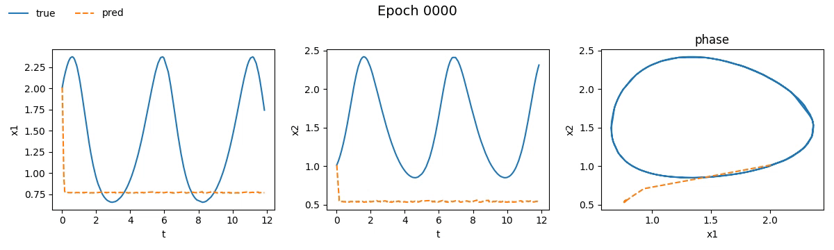
Figure 2. Training on Lotka-Volterra with SimpleNet
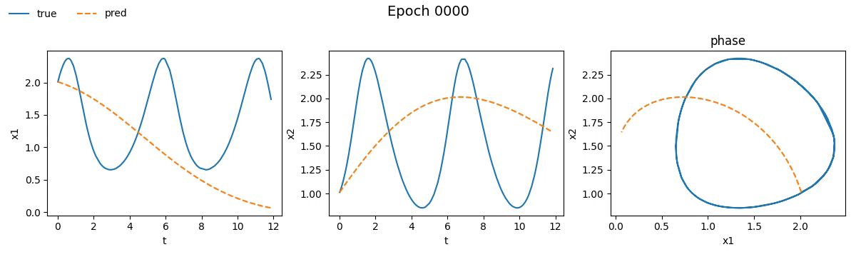
Figure 3. Training on Lotka-Volterra with NODE
Even from these gifs, it’s clear that with just \(100\) epochs, the NODE appears to have
grasped the dynamics much better than SimpleNet. But training alone isn't enough.
Let's now see how these models perform when we test them outside the training range.
Forecast
During training, we taught or at least tried to teach, the NODE and SimpleNet models to follow the behavior of a
dynamic system. Yes, it was the Lotka-Volterra system, but the networks don’t know that. All they saw was a
list of randomly sampled values over time. But how can we verify whether they actually understood
anything? For all we know, they might have just memorized the train and test sets without being able
to generalize. What we want to verify is:
Given samples from \((0, \, 12)\) seconds, can I predict the behavior beyond \(12\) seconds?
To do this, we need to proceed in two different ways for SimpleNet and NODE. That’s because while
forward prediction is implicit for NODEs, it’s not for traditional networks. For SimpleNet, then,
we use an autoregressive approach, feeding the predicted state back in as input to estimate the next state.
Let’s take a look at what that means in code:
@torch.no_grad()
def predict_mlp(model, loader) -> tuple[np.ndarray, np.ndarray]:
    ...
    x = x_i[0]
    for k in range(t_grid.size(0)-1):
        dt = t_grid[k+1]-t_grid[k]
        x = model(x, dt)
        traj.append(x)
    pred = np.stack(traj, 0)
    ...
    return pred, tgt

@torch.no_grad()
def predict_node(model, loader) -> tuple[np.ndarray, np.ndarray]:
    ...
    x0 = x_i[0]
    traj = odeint(model, x0, t_grid, method=model.method)
    ...
    return traj, tgt
In the predict_mlp function, used for making predictions with SimpleNet, we start with an initial value say,
the state \(x\) at \(t = 12\) seconds. We make a prediction using \(x\) as input and moving forward by a
time \(dt\). The output, i.e. the state at time \(dt\), is then used as the input to predict the state at
the next \(dt\). Since we want predictions over the range \((12, 18)\) seconds, this loop
continues until we reach \(t = 18\). This kind of iterative prediction is fragile: each error
propagates over time, making generalization harder.
As for the NODE, it makes things much simpler. Because of its very nature, when we integrate from \(12\) to \(18\)
seconds, we’re computing the dynamics, and thus all the states within that time window.
In practice, it’s enough to call odeint once with all the time steps in the desired range, and the
model returns the entire predicted trajectory. But enough talk, let’s see how our networks actually performed
in predicting the future.

Figure 4. Lotka-Volterra Forecast with SimpleNet

Figure 5. Lotka-Volterra Forecast with NODE
From the training videos, it was already clear that SimpleNet didn’t perform particularly well.
And looking at the forecast, we can safely say it didn’t get a thing its forecast is, frankly, atrocious by the
second step. On the other hand, NODE seems to have grasped the dynamics quite well, as it manages to make
accurate predictions for all states over a very wide time window.
In conclusion, the NODE not only showed it could fit the data well,
but also generalized effectively to a time window it had never seen before.
Sure, NODEs take longer, but as someone once said: quality comes at a price.
The Harmonic Oscillator
The second problem tackled is the harmonic oscillator. I won’t go over all the steps again since they are essentially the same as those above, just with different data. In this paragraph, I’ll simply explain how I transitioned from a physical problem to a mathematical model, and we’ll look only at the forecasting results.
Let’s start with the classic physics exercise involving a mass attached to a spring, as shown in the image below.
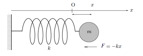
Figure 6. Mass Attached to a Spring
If you try to pull and release the mass, it will oscillate around its equilibrium point until it returns to the stable state where it's at rest. This motion is called a harmonic oscillator. Let’s look at the physical laws behind it. From Newton’s law, we know that force equals mass times acceleration. But what is acceleration? From Part 1, we know that velocity is the first derivative of position with respect to time. Since acceleration is the first derivative of velocity with respect to time, we then have that acceleration is the second derivative of position with respect to time.
In the image above, we do have a notion of position. It’s the distance between the mass \(m\) and its equilibrium point, denoted by \(x\). So we write:
But from Hooke’s Law we know that the elastic force is a force opposite to the displacement, dependent on the spring’s elastic constant \(k\) and the displacement itself. So we can write:
Thus, if there are no other forces at play, the total force is just the elastic component. Hence:
Now suppose the mass is sitting on a plastic floor that introduces significant friction. By definition, a frictional force is equal to velocity times a friction coefficient. Velocity, as we’ve said, is the first derivative of position with respect to time. Moreover, since it’s a dissipative force, it subtracts energy from the system. Therefore, we write:
Including this force in the system, we now have:
Which simplifies to:
Let’s define:
Where \(\omega^2\) is called the natural frequency of the oscillator, and \(\gamma\) the damping coefficient. So:
We've reached the differential form of the harmonic oscillator. But we’re not done yet, because ODESolvers can only handle first-order differential equations, so as it is, this equation isn’t usable. Let’s leverage a property of differential equations, specifically the one that says:
Any ordinary differential equation of order \(n\) can be rewritten as an equivalent system of \(n\) first-order equations.
We’ll make a simple change of variables:
After this change of variables, we can write the second-order differential equation as two first-order differential equations:
This is a form that an ODESolver can handle, and it represents the dynamics we need to solve. In code, this dynamic system becomes:
class HarmonicOscillator(DatasetProvider):

    def __init__(self, n_train: int = 80, noise_std: float = 0.01, t_train_range: tuple[float, float] = (0.0, 10.0),
                 t_extra_range: tuple[float, float] = (10.0, 15.0), n_extra: int = 200, n_resamp: int = 200, omega: float = 1.0,
                 gamma: float = 0.1, initial_values: tuple[float, float] = (2.0, 0.0)) -> None:
        super().__init__(initial_values=initial_values, n_train=n_train, noise_std=noise_std,
                         t_train_range=t_train_range, t_extra_range=t_extra_range, n_extra=n_extra,
                         n_resamp=n_resamp)

        self.omega = float(omega)
        self.gamma = float(gamma)

    ...

    def dynamics(self, t: torch.Tensor, state: torch.Tensor) -> torch.Tensor:
        x1, x2 = state[0], state[1]
        x1dt = x2
        x2dt = -(self.omega ** 2) * x1 - self.gamma * x2
        return torch.stack([x1dt, x2dt])

    ...
The rest, as they say, is history. So I'll just show the forecast plots:
 Figure 7. Harmonic Oscillator Forecast with
 SimpleNet
 Figure 8. Harmonic Oscillator Forecast with
 NODE
From these plots we can see that, once again, the NODE seems to have truly captured the dynamics, while the classic network looks a bit confused.
So to sum it all up, NODEs have proven their potential—especially in contexts involving continuous dynamics.
Are they slow? Yes.
Are they heavy to integrate? Definitely.
Are they hard to tune? Also true.
But they do learn how a system evolves, and they do it well. With constant memory usage, simpler architectures, and a remarkable ability to generalize.
To Wrap Up
We finally wrap up this series of articles on NODEs. It's been a long and, let's be honest, exhausting journey, for both you and me. But hey, we walk away with a nice bundle of knowledge, right? Before closing, I’d like to dot a few i’s on a couple of points. Starting with classic neural networks, which might have seemed a bit neglected here. That’s not really the case. To keep the comparison fair, I used just one training approach, but with the proper tuning, a classic network can perform really well. Now, about NODEs. Yes, this article series is over, but NODEs are just the foundation. The ones that started it all. In this series, I used them for forecasting, but just like classic networks, they can be used for classification, regression, generation... And beyond that: NODEs have inspired many other fascinating architectures. From CNFs for image generation, to Liquid Neural Networks used in robotics and control, and even to Physics-Informed Neural Networks (Lagrangian Nets, Hamiltonian Nets, etc.), which integrate physics to model complex systems. In short, there’s a lot more out there. And each of these deserves its own deep dive. Who knows, maybe one day I’ll hit you with that too.
That said, as always, I invite you to check out the full code here and give it a spin yourself.
Until next time.